Coherent Structures from Spatio-Temporal Frequency Responses
At first view, turbulent flows look 'statistical’, i.e. random and unorganized. Depending on the flow conditions and geometry, there are however multitudes of organized flow structures buried in this randomness. They are commonly referred to as coherent structures. One effective technique to dig them out of the random mess is to look for peaks in the spatio-temporal power spectral densities of flow velocity or vorticity fields. This kind of 'data mining’ is done on the results of Direct Numerical Simulations (DNS) data of the full Navier-Stokes equations. If on the other hand one deals with only the Linearized Navier-Stokes (LNS) equations (linearized around some mean or laminar flow condition, not to be confused with just the Stokes equations), then one can obtain the power spectral densities -in a 'simulation-free’ manner- from computations of the spatio-temporal frequency response. In this setting, coherent structures in turbulent flow correspond to the most resonant structures when the flow is excited by random body forces.
Input-output analysis of the linearized Navier-Stokes equations
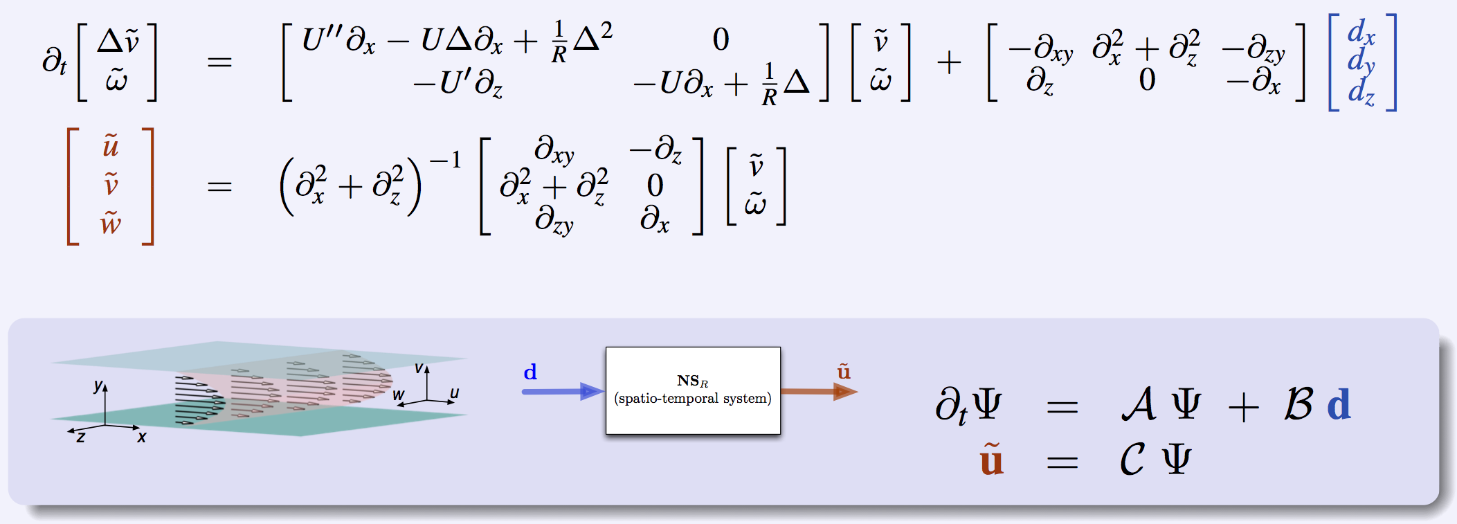 |
In the above setting, the LNS around laminar Poiseuille flow with body forces as inputs are shown. This is an input-output view of the flow dynamics with the 'disturbance’ body force field  as input, and flow field fluctuations (around laminar)
  as the output. All fields are spatio-temporal signals. Even if the body force field has no structure (i.e. is a white spatio-temporal random field), the output will have a lot of structure inherited from the dynamics of the LNS.
Component-wise view of the spatio-temporal frequency response
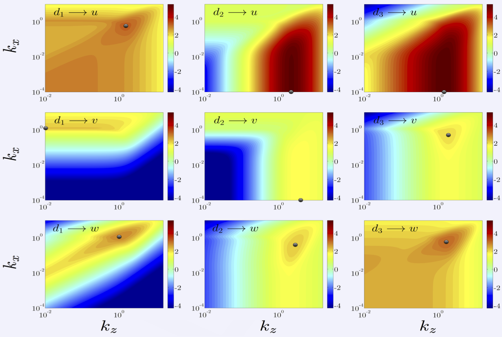 |
The 3x3 matrix of spatio-temporal frequency responses from each of the polarized body forces ( ) to each of the components of the channel flow field fluctuations (
 ,
, ,
, ). This frequency response is a large object! Due to translation invariance of the dynamics in time (
 ), streamwise (
 ) and spanwise (
 ) directions, it is an operator-valued function
  of the temporal (
 ), streamwise (
 ) and spanwise (
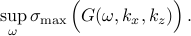
 ) frequency and wave numbers. The plots above are made easier to visualize by maxing over temporal frequency and wall-normal effects, i.e. by plotting
Note that if we integrate in and take a square-sum rather than a max of singular values, we get qualitatively similar plots. The above plots correspond to the spatio-temporal power spectral densities one would find if the LNS are excited by white random field body forces. However, they are computed here using singular values of an operator-valued function rather than a stochastic simulation!
The upper-right two components (from  ,
,  to
to  ) are by far the biggest (they scale with
  , while all other subsystems scale with
  ). Their maxima are achieved near
  and
and 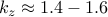 . These spatio-temporal resonances are fundamental! Their structure is shown below.
The most 'resonant’ flow structures
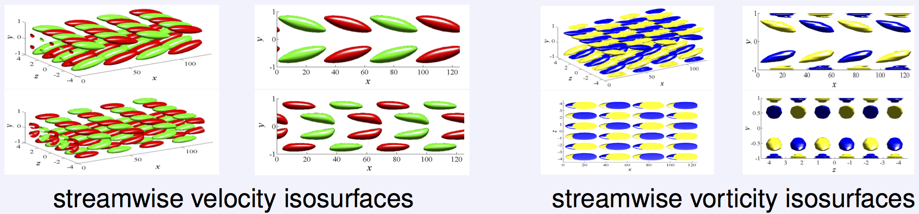 |
Isosurface plots of the most resonant flow structures according to the frequency response above. Note the greatly compressed streamwise axis scale. These structures are very long, alternating high and low streamwise velocity 'streaks’, interwoven with counter-rotating streamwise vortices.
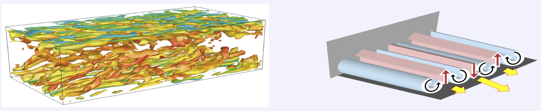
Comparison with DNS data
 |
Related Papers
Componentwise Energy Amplification in Channel Flows, M. Jovanovic and B. Bamieh, J. Fluid Mechanics, 2005.
Energy Amplification in Channel Flows with Stochastic Excitation, B. Bamieh and M. Dahleh, Physics of Fluids, 2001.