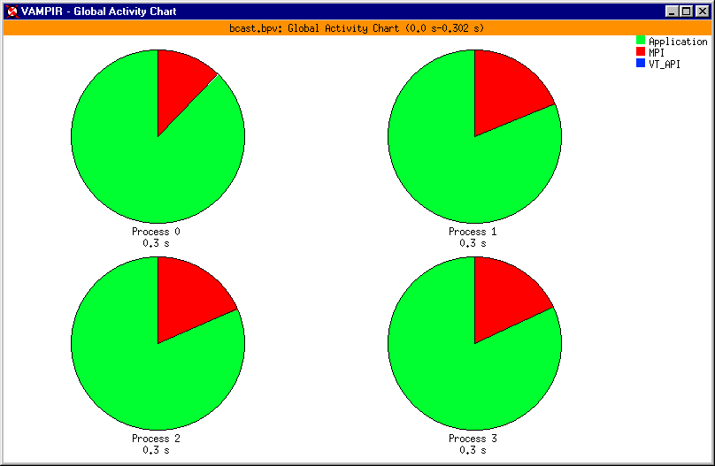
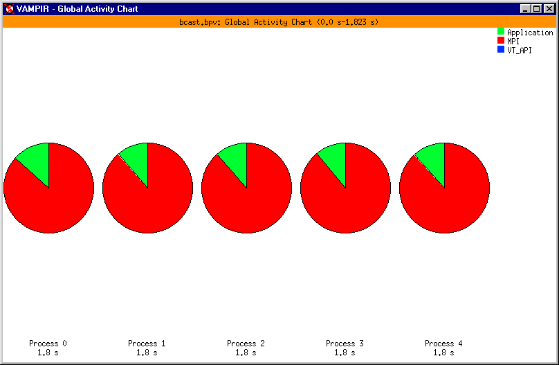
Application work vs. MPI communication
Executing the parallel Gauss elimination program on a 300 by 300 symmetric matrix, 3, 4 and 5 processors are used, respectively, to compare the performance. The optimization task for a parallel program is to speed up the computation, which requires the balance of the number of processors involved (prefers more processors) and the communication time consumed (prefers less processors). From the following data, we can see that for a 300 by 300 symmetric matrix, 4 processors can give satisfactory results whereas the computation is slowed down if 5 processors are used (since much more time is spent on MPI communication). It is clear that more processors should to be used if the matrix size is enlarged.
Case I: 3 processors
Program running time: (in seconds):
processor 0 = 0.3388819695,
processor 1 = 0.3543879986,
processor 2 = 0.3539350033.
The Activity Chart display window: With the default pie chart display you can recognize the load imbalance at a glance in the traced
program by comparing the different time consumption of activities over all processes. VAMPIR can assist
the user by visualizing the actual trace data in different chart modes. Depending on the users
preference the activity chart can be switched to the so called "Histogram" mode.
To focus on a single activity, for instance MPI, please open the context menu with
the right mouse button click inside the Activity Chart and select the activity MPI from the Display menu
cascade. A new set of pie charts is drawn, showing only the symbols of the selected activity MPI. So you
can compare different activities or symbols of all processes.

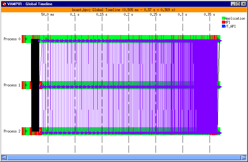
The Global Timeline display widow: For each process, the display shows the different states and their change over execution time
along a horizontal time axis. Messages between processes are indicated as lines connecting the
sending and receiving processes.
By default, the timeline view shows the whole execution trace. Even with smaller traces this will
lead to a cluttered display like that shown in the figure below. To concentrate on a special part of
the trace file please invoke the VAMPIR zooming function by selecting an area of interest with your
mouse. To zoom into a part of the timeline view, move the the mouse pointer to the start of the
interval you want to zoom into, press the left mouse button, drag the mouse to the
end of the zoom interval while keeping the left mouse button down (only the x-coordinate matters).
VAMPIR will indicate the marked region with rubber-bands. Finally, release the mouse button. The
timeline display will be redrawn showing just the time interval you selected, with the contents
magnified accordingly.
You can repeatedly zoom into arbitrary levels of detail. Zooming out step-by-step can be done
with the Undo Zoom function of the context menu.
The Global Displays/Timeline view is the central display of VAMPIR because all other global and process
specific statistic displays can be configured to use only the portion of time the timeline view
displays. This option can be selected for a single display by selecting Timeline from
the appropriate context menu.
Case II: 4 processors
Program running time: (in seconds):
processor 0 = 0.2572540045,
processor 1 = 0.2717200518,
processor 2 = 0.2717679739,
processor 3 = 0.2718409300.
The Activity Chart display window:
The Global Timeline display widow:

Case III: 5 processors
Program running time (in seconds):
processor 0 = 1.801327109,
processor 1 = 1.814256072,
processor 2 = 1.823287964,
processor 3 = 1.821319938,
processor 4 = 1.822461009.
The Activity Chart display window:
The Global Timeline display widow:
