Figure 1.3:

Output of a stochastic system versus time.

Code for Figure 1.3

Text of the GNU GPL.

main.py

 1
 2
 3
 4
 5
 6
 7
 8
 9
10
11
12
13
14
15
16
17
18
19
20
21
22
23
24
25
26
27
28
29
30
31
32
33
34
35
36
37
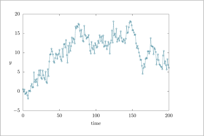
# Example noisy dataset.
import numpy as np
import matplotlib.pyplot as plt
from misc import gnuplotsave
import os

# Example noisy dataset
a = 1
c = 1
r = 1
q = 1

x0 = 1
q0 = 1

nsim = 201
x = np.zeros(nsim + 1) # Add 1 for Python indexing
y = np.zeros(nsim)
t = np.arange(nsim)

np.random.seed(0)
x[0] = x0 + np.sqrt(q0)*np.random.randn()

for i in range(nsim):
    y[i] = c*x[i] + np.sqrt(r)*np.random.randn()
    x[i + 1] = a*x[i] + np.sqrt(q)*np.random.randn()

if not os.getenv('OMIT_PLOTS') == 'true':
    plt.figure(figsize=(8,6))
    plt.plot(t, y, '-o', markersize=2)
    plt.grid(True)
    plt.savefig('noisy.png')
    plt.close()

# Save data to file
output = np.column_stack((t, y))
gnuplotsave('noisy.dat', output)