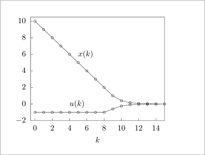
Figure 2.1:

Example of MPC.

Code for Figure 2.1

Text of the GNU GPL.

main.py

 1
 2
 3
 4
 5
 6
 7
 8
 9
10
11
12
13
14
15
16
17
18
19
20
21
22
23
24
25
26
27
28
29
30
31
32
33
34
35
36
37
38
39
40
41
42
43
44
45
46
47
48
49
50
51
52
53
54
55
56
57
58
59
60
61
62
63
64
65
66
67
68
69
70
71
72
#
# compute simple LQ MPC solution
# jbr, 8/13/2008
#
import numpy as np
from numpy.linalg import inv
import matplotlib.pyplot as plt
import os

# compute simple LQ MPC solution
# jbr, 8/13/2008

A = 1
B = 1
Q = 1
R = 1
N = 2

H = np.array([[3, 1], [1, 2]])
uub = np.ones((N,1))
ulb = -uub

def control_law(x):
    uN = -inv(H) @ np.array([[2],[1]]) * x
    uN = np.minimum(uN, uub)
    uN = np.maximum(uN, ulb)
    return uN[0, 0]

T = 15
# Closed-loop simulation
x0 = 10
x = np.zeros((1,T+1))
x[0,0] = x0
u = np.zeros((1,T+1))
time = np.arange(T+1)

for k in range(T+1):
    u[0,k] = control_law(x[0,k])
    if k == T:
        break
    x[0,k+1] = A*x[0,k] + B*u[0,k]

# Evaluate control law
xmin = -3
xmax = -xmin
nxs = 100
xvec = np.linspace(xmin, xmax, nxs).reshape(-1,1)

uvec = np.zeros(nxs)
for i in range(nxs):
    uvec[i] = control_law(xvec[i])
uvec = uvec.reshape(-1,1)

if not os.getenv('OMIT_PLOTS') == 'true':
    plt.figure(1)
    plt.plot(time, np.vstack((x,u)).T, '-o')
    plt.axis([0,T,-2,10])

    plt.figure(2)
    plt.plot(xvec, uvec)
    plt.axis([xmin, xmax, 2*ulb[0], 2*uub[0]])

    plt.show(block=False)

# Save data
data1 = np.column_stack((time, x.T, u.T))
data2 = np.column_stack((xvec, uvec))

np.savetxt('lqmpc.dat', data1, header='time x u', comments='# ')
with open('lqmpc.dat', 'a') as f:
    f.write('\n\n')
    np.savetxt(f, data2, header='xvec uvec', comments='# ')