Figure 2.8

Figure 2.8:

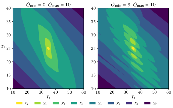
Feasible sets \mathcal {X}_N for two values of \dot {Q}_min. Note that for \dot {Q}_min=9 (right-hand side), \mathcal {X}_N for N \leq 4 are disconnected sets.

Code for Figure 2.8

getcooler.py


 1
 2
 3
 4
 5
 6
 7
 8
 9
10
11
12
13
14
15
16
17
18
19
20
21
22
23
24
25
26
27
28
29
30
31
32
33
34
35
36
37
38
39
40
41
42
43
44
45
46
47
48
49
50
51
52
53
54
55
56
57
58
59
60
61
62
63
64
65
66
67
68 # sys = getcooler()
#
# Returns a struct of parameters for the cooler system.
import numpy as np
from scipy.linalg import expm, solve_discrete_lyapunov

def getcooler():
    """
    sys = getcooler()

    Returns a struct of parameters for the cooler system.
    """
    # Input validation
    if len(locals()) > 0:
        raise ValueError('Function takes no input arguments')

    # Define system
    Nx = 2
    Nu = 2
    alpha = 2
    beta = 1
    rho1 = 1
    rho2 = 1

    ns = np.array([0, 1, 2])
    Qmin = 9
    Qmax = 10

    nss = 1
    Qss = nss*Qmax

    uss = np.array([[Qss], [nss]])

    T0 = 40
    T1ss = 35
    T2ss = 25

    xss = np.array([[T1ss], [T2ss]])

    # Continuous-time system
    a = np.array([[-alpha - rho1, rho1],
                  [rho2, -rho2]])
    b = np.array([[0, 0],
                  [-beta, 0]])
    f = np.array([[alpha*T0],
                  [0]])

    # Discretize
    Delta = 0.25
    A = expm(Delta*a)
    B = np.linalg.solve(a, (A - np.eye(2)) @ b)
    F = np.linalg.solve(a, (A - np.eye(2)) @ f)

    # Choose penalty
    Q = np.eye(Nx)
    R = np.eye(Nu)

    # Pick terminal region
    Xf = {'rho': 1, 'P': solve_discrete_lyapunov(A.T, Q)}  # Level set for Xf

    # Save everything to a dict
    sys = {}
    local_vars = locals()
    for var in list(local_vars.keys()):
        if var != 'sys':
            sys[var] = local_vars[var]

    return sys

main.py


  1
  2
  3
  4
  5
  6
  7
  8
  9
 10
 11
 12
 13
 14
 15
 16
 17
 18
 19
 20
 21
 22
 23
 24
 25
 26
 27
 28
 29
 30
 31
 32
 33
 34
 35
 36
 37
 38
 39
 40
 41
 42
 43
 44
 45
 46
 47
 48
 49
 50
 51
 52
 53
 54
 55
 56
 57
 58
 59
 60
 61
 62
 63
 64
 65
 66
 67
 68
 69
 70
 71
 72
 73
 74
 75
 76
 77
 78
 79
 80
 81
 82
 83
 84
 85
 86
 87
 88
 89
 90
 91
 92
 93
 94
 95
 96
 97
 98
 99
100
101
102
103
104
105
106
107
108
109
110
111
112
113
114
115
116
117
118
119
120
121
122
123
124
125
126
127
128
129
130
131
132
133
134
135
136
137
138
139
140
141
142
143
144
145
146
147
148
149
150
151
152
153
154
155
156
157
158
159
160
161
162
163
164
165
166
167
168
169
170
171
172
173
174
175
176
177
178
179
180
181
182 # [depends] functions/getcooler.py
# [makes] coolerXn.mat

# Calculation of X_n sets for a linear system with discrete actuators.
# Note that for computational purposes, we use a polyhedral approximation of
# the true elliptical X_n.

import sys
import os
import numpy as np
sys.path.append('functions/')
from scipy import linalg
from scipy import io
import matplotlib.pyplot as plt
from getcooler import getcooler
from scipy.spatial import ConvexHull
import pickle

sys = getcooler()
Qmax = sys['Qmax']
Qmin = sys['Qmin']
ns = sys['ns']
A = sys['A']
B = sys['B'][:,0].reshape(-1,1)  # Second input doesn't affect dynamics
F = sys['F']
P = sys['Xf']['P']
xss = sys['xss']
rho = sys['Xf']['rho']

def ellipseterm(A, P, xss, rho, n):
    """
    Returns a polyhedral tangent approximation of an ellipsoidal terminal set.
    Also makes a plot of the evolution of Xf under A.

    Xf is a 2 by n matrix of extreme points. A and b are the polyhedral
    representation of Xf. P is the terminal penalty weight.
    """
    if not (isinstance(n, int) and n > 0):
        raise ValueError("n must be positive integer")

    eigvals, eigvecs = linalg.eigh(P/rho)

    a = 1/np.sqrt(eigvals[0])
    b = 1/np.sqrt(eigvals[1])

    def calc(t):
        return np.vstack((eigvecs[0,0]*a*np.cos(t) + eigvecs[0,1]*b*np.sin(t),
                         eigvecs[1,0]*a*np.cos(t) + eigvecs[1,1]*b*np.sin(t)))

    T = np.linspace(0, 2*np.pi, n+1)
    t = np.linspace(0, 2*np.pi, 10*n+1)

    E = calc(T)
    AE = A @ E

    e = calc(t)
    Ae = A @ e

    if not os.getenv('OMIT_PLOTS') == 'true':
        plt.figure()
        plt.plot(E[0,:] + xss[0], E[1,:] + xss[1], '-ob', label='X_f')
        plt.plot(e[0,:] + xss[0], e[1,:] + xss[1], '--b')
        plt.plot(AE[0,:] + xss[0], AE[1,:] + xss[1], '-or',
                 label='f(X_f, \\kappa_f(X_f))')
        plt.plot(Ae[0,:] + xss[0], Ae[1,:] + xss[1], '--r')
        plt.xlabel('T_1')
        plt.ylabel('T_2')
        plt.title('Terminal Region X_f = {x | x\'Px <= ' + str(rho) + '}')
        plt.legend(loc='upper right')

    return xss.reshape(-1,1) + E[:,:-1]

Xf = ellipseterm(A, P, xss, rho, 32)

def addpoints(p1, p2):
    """Adds two arrays of points (2D with rows x and y)."""
    p = p1.reshape(p1.shape[0], p1.shape[1], 1) + p2.reshape(p2.shape[0], 1, p2.shape[1])
    psize = p.shape
    return p.reshape(psize[0], psize[1]*psize[2])

def minkowski(p1, p2=None):
    """
    Returns minkowski sum of extreme point polytopes p and q.
    Only works for two dimensions.
    """
    if p2 is None:
        p2 = np.zeros((2,1))

    p = addpoints(p1, p2)
    ch = ConvexHull(p.T)
    return p[:,ch.vertices]

def calcXn(A, B, f, N, Xf, U, x0=None):
    """
    Calculate X_n sets for the system

        x^+ = Ax + Bu + f

    Xf should be an extreme point representation of Xf, and U should be a
    list of extreme-point polytopes for U.
    """
    Ainv = linalg.inv(A)
    BU = [B @ u + f for u in U]
    Xn = [None]*(N+1)
    Xn[0] = [Xf]

    print(f'*** Calculating Xk (max k = {N}) ***')
    for n in range(1,N+1):
        Xn[n] = []
        for xn in Xn[n-1]:
            for bu in BU:
                Xn[n].append(Ainv @ minkowski(xn, -bu))
        print(f'   k = {n}: {len(Xn[n])} regions')

    return Xn

# Calculate feasible sets
Ucontinuous = [np.array([[0, max(ns)*Qmax]])]
Udiscrete = [n*np.array([[Qmin, Qmax]]) for n in ns]

N = 7
Xc = calcXn(A, B, F, N, Xf, Ucontinuous)
Xd = calcXn(A, B, F, N, Xf, Udiscrete)

def plotXn(Xn, lims=None):
    """Plots a set of regions on the current axes."""
    if os.getenv('OMIT_PLOTS') == 'true':
        return

    if lims is not None:
        plt.axis(lims)

    colors = plt.cm.viridis(np.linspace(0,1,len(Xn)))[::-1]

    for n in range(len(Xn)-1,-1,-1):
        xn = Xn[n]
        for i in range(len(xn)):
            plt.fill(xn[i][0,:], xn[i][1,:], color=colors[n],
                    edgecolor='none', zorder=-n)

    plt.xlabel('T_1')
    plt.ylabel('T_2')

lims = np.hstack( ((sys['T1ss'] + 25*np.array([-1, 1])),
                  (sys['T2ss'] + 15*np.array([-1, 1]))) )

if not os.getenv('OMIT_PLOTS') == 'true':
    print('Plotting. May take some time.')
    plt.figure()

    plt.subplot(121)
    plotXn(Xc, lims)
    plt.title('Q_{min} = 0, Q_{max} = 10')

    plt.subplot(122)
    plotXn(Xd, lims)
    plt.title('Q_{min} = 9, Q_{max} = 10')

# Convert each 'listed' array to just an array
def to_cellarray(pylist):
    """Convert a Python list of arrays/lists into a MATLAB cell-array-like object array."""
    cell = np.empty((len(pylist),), dtype=object)
    for i, elem in enumerate(pylist):
        if isinstance(elem, (list, tuple)):
            cell[i] = to_cellarray(elem)  # recursive wrap
        else:
            cell[i] = np.asarray(elem)
        obj = np.empty(len(cell), dtype=object)
        for i, arr in enumerate(cell):
            obj[i] = arr
    return cell

Xdf = to_cellarray(Xd)
Xcf = to_cellarray(Xc)

data = {
    'continuous': Xcf,
    'discrete': Xdf,
    'lims': lims
}

io.savemat('coolerXn.mat', data, 5)