Figure 3.8

Figure 3.8:

Concentration versus time for the ancillary model predictive controller with sample time \Delta =12 (left) and \Delta =8 (right).

Code for Figure 3.8

cstrparam.py


 1
 2
 3
 4
 5
 6
 7
 8
 9
10
11
12
13
14
15
16
17
18
19
20
21
22
23
24
25
26
27
28
29
30
31
32
33
34
35
36
37
38
39
40
41
42
43
44
45
46
47
48
49
50
51
52
53
54
55
56
57
58
59
60
61
62
63
64
65
66
67
68 # Loads default parameters for robust MPC CSTR problem.
# Model Parameters.
import numpy as np

def cstrparam(Nsim=None):
    pars = {}

    # Model Parameters
    pars['theta'] = 20
    pars['k'] = 300
    pars['M'] = 5
    pars['xf'] = 0.3947
    pars['xc'] = 0.3816
    pars['alpha'] = 0.117

    # Simulation
    pars['tfinal'] = 300
    pars['N'] = 40
    pars['Q'] = 1/2
    pars['R'] = 1/2
    pars['Qf'] = 1e5
    pars['Nx'] = 2
    pars['Nu'] = 1
    pars['Np'] = 1
    pars['Delta'] = 3
    pars['xub'] = np.array([[2], [2]])
    pars['xlb'] = np.array([[0], [0]])
    pars['uub'] = 2
    pars['ulb'] = 0
    pars['colloc'] = 5
    pars['plantSteps'] = 2

    # Initial Conditions and Setpoints
    pars['x0'] = np.array([[0.9831], [0.3918]])
    pars['ze'] = np.array([[0.2632], [0.6519]])
    pars['uprev'] = 0.02
    pars['usp'] = 455/600

    # Nominal constraints
    pars['uub_nominal'] = 2
    pars['ulb_nominal'] = 0.02
    pars['A'] = 0
    pars['w'] = 1

    def cstrode(x, u, p, pars):
        # Extract states
        c = x[0]
        T = x[1]
        t = x[2] if len(x) > 2 else 0  # Handle optional time state

        # Calculate reaction rate and disturbance
        rate = pars['k'] * c * np.exp(-pars['M'] / T)
        w = pars['A'] * np.sin(t * pars['w']) * p

        # State derivatives
        dcdt = (1 - c) / pars['theta'] - rate
        dTdt = (pars['xf'] - T) / pars['theta'] + rate - pars['alpha'] * u * (T - pars['xc']) + w
        dtdt = 1

        return np.array([dcdt, dTdt, dtdt])

    # Add ODE function to parameters
    pars['ode'] = cstrode

    # Set random seed
    np.random.seed(0)

    return pars

nominalmpc.py


  1
  2
  3
  4
  5
  6
  7
  8
  9
 10
 11
 12
 13
 14
 15
 16
 17
 18
 19
 20
 21
 22
 23
 24
 25
 26
 27
 28
 29
 30
 31
 32
 33
 34
 35
 36
 37
 38
 39
 40
 41
 42
 43
 44
 45
 46
 47
 48
 49
 50
 51
 52
 53
 54
 55
 56
 57
 58
 59
 60
 61
 62
 63
 64
 65
 66
 67
 68
 69
 70
 71
 72
 73
 74
 75
 76
 77
 78
 79
 80
 81
 82
 83
 84
 85
 86
 87
 88
 89
 90
 91
 92
 93
 94
 95
 96
 97
 98
 99
100
101
102
103
104
105 # reference_trajectory = nominalmpc(pars)
#
# Runs nominal NMPC for CSTR example in Chapter 3 to generate the reference
# trajectory for tube-based MPC.
#
# Note: In this script, "p" denotes the disturbance ("w" in MPC textbook).
import numpy as np
import mpctools as mpc


def nominalmpc(pars):
    Nu     = pars['Nu']
    Np     = pars['Np']
    Delta  = pars['Delta']
    tfinal = pars['tfinal']
    N      = pars['N']
    uprev  = pars['uprev']
    usp    = pars['usp']
    colloc = pars['colloc']
    Q      = pars['Q']
    R      = pars['R']
    Qf     = pars['Qf']

    # Augmented state includes time as third component.
    Nx  = pars['Nx'] + 1
    xub = np.append(pars['xub'].flatten(), np.inf)
    xlb = np.append(pars['xlb'].flatten(), -np.inf)
    x0  = np.append(pars['x0'].flatten(), 0.0)
    ze  = np.append(pars['ze'].flatten(), tfinal)

    # Tightened constraints for nominal problem.
    uub = pars['uub_nominal']
    ulb = pars['ulb_nominal']

    def ode_model(x, u):
        return pars['ode'](x, u, 0, pars)

    def ode_plant(x, u, p):
        return pars['ode'](x, u, p, pars)

    def stagecost(x, u, x_sp, u_sp):
        xerr = x[:pars['Nx']] - x_sp[:pars['Nx']]
        uerr = u - u_sp
        return Q * (xerr @ xerr) + R * (uerr @ uerr)

    def termcost(x, x_sp):
        xerr = x[:pars['Nx']] - x_sp[:pars['Nx']]
        return Qf * (xerr @ xerr)

    ode_casadi = mpc.getCasadiFunc(ode_model, [Nx, Nu], ['x', 'u'], 'cstr_model')
    cstrsim    = mpc.getCasadiIntegrator(ode_plant, Delta, [Nx, Nu, Np],
                                         ['x', 'u', 'p'], 'cstr_plant')
    l  = mpc.getCasadiFunc(stagecost, [Nx, Nu, Nx, Nu], ['x', 'u', 'x_sp', 'u_sp'], 'l')
    Pf = mpc.getCasadiFunc(termcost,  [Nx, Nx],          ['x', 'x_sp'],               'Pf')

    # Controller dimensions and collocation.
    N_dict = {'x': Nx, 'u': Nu, 't': N, 'c': colloc}

    # Constant setpoints over the horizon.
    xsp_init = np.tile(ze, (N + 1, 1))      # (N+1, Nx)
    usp_init = np.full((N, Nu), usp)        # (N, Nu)

    # Initial guess: linear interpolation to setpoint.
    guess_x = np.column_stack([
        np.linspace(x0[0], ze[0], N + 1),
        np.linspace(x0[1], ze[1], N + 1),
        np.linspace(x0[2], x0[2] + N * Delta, N + 1),
    ])  # (N+1, Nx)
    guess_u = np.linspace(uprev, usp, N).reshape(N, Nu)  # (N, Nu)

    solver = mpc.nmpc(
        f=ode_casadi,
        N=N_dict,
        Delta=Delta,
        verbosity=0,
        l=l,
        Vf=Pf,
        x0=x0,
        guess={'x': guess_x, 'u': guess_u},
        par={'xsp': xsp_init, 'usp': usp_init},
        lb={'x': xlb, 'u': np.full(Nu, ulb)},
        ub={'x': xub, 'u': np.full(Nu, uub)},
        inferargs=True,
    )

    # Closed-loop simulation.
    Nsim = int(tfinal / Delta) + N
    x = np.full((Nx, Nsim + 1), np.nan)
    u = np.full((Nu, Nsim), np.nan)
    x[:, 0] = x0

    for i in range(Nsim):
        solver.fixvar('x', 0, x[:, i])
        solver.solve()
        print(f'{i}: {solver.stats["status"]}')
        if solver.stats['status'] != 'Solve_Succeeded':
            print(f'Warning: failed at step {i}!')
            break

        u[:, i] = np.array(solver.var['u', 0]).flatten()
        x[:, i + 1] = np.array(cstrsim(x[:, i], u[:, i], np.zeros(Np))).flatten()
        solver.saveguess()

    t = Delta * np.arange(Nsim + 1)
    return {'x': x, 'u': u, 't': t}

tubempc.py


  1
  2
  3
  4
  5
  6
  7
  8
  9
 10
 11
 12
 13
 14
 15
 16
 17
 18
 19
 20
 21
 22
 23
 24
 25
 26
 27
 28
 29
 30
 31
 32
 33
 34
 35
 36
 37
 38
 39
 40
 41
 42
 43
 44
 45
 46
 47
 48
 49
 50
 51
 52
 53
 54
 55
 56
 57
 58
 59
 60
 61
 62
 63
 64
 65
 66
 67
 68
 69
 70
 71
 72
 73
 74
 75
 76
 77
 78
 79
 80
 81
 82
 83
 84
 85
 86
 87
 88
 89
 90
 91
 92
 93
 94
 95
 96
 97
 98
 99
100
101
102
103
104
105
106
107
108
109
110
111
112
113
114
115
116
117
118
119
120
121
122
123 # result = tubempc(pars)
#
# Runs tube-based NMPC for CSTR example in Chapter 3.
#
# Note: In this script, "p" denotes the disturbance ("w" in MPC textbook).
import numpy as np
import mpctools as mpc


def tubempc(pars):
    Nu         = pars['Nu']
    Np         = pars['Np']
    Delta      = pars['Delta']
    uub        = pars['uub']
    ulb        = pars['ulb']
    tfinal     = pars['tfinal']
    N          = pars['N']
    plantSteps = pars['plantSteps']
    colloc     = pars['colloc']
    Q          = pars['Q']
    R          = pars['R']
    Qf         = pars['Qf']

    # Augmented state includes time as third component.
    Nx  = pars['Nx'] + 1
    xub = np.append(pars['xub'].flatten(), np.inf)
    xlb = np.append(pars['xlb'].flatten(), -np.inf)
    x0  = np.append(pars['x0'].flatten(), 0.0)

    # Reference trajectories from nominal MPC.
    xsp = pars['reftraj']['x']   # (Nx, Nsim_nom+1)
    usp = pars['reftraj']['u']   # (Nu, Nsim_nom)

    def ode_model(x, u):
        return pars['ode'](x, u, 0, pars)

    def ode_plant(x, u, p):
        return pars['ode'](x, u, p, pars)

    def stagecost(x, u, x_sp, u_sp):
        xerr = x[:pars['Nx']] - x_sp[:pars['Nx']]
        uerr = u - u_sp
        return Q * (xerr @ xerr) + R * (uerr @ uerr)

    def termcost(x, x_sp):
        xerr = x[:pars['Nx']] - x_sp[:pars['Nx']]
        return Qf * (xerr @ xerr)

    ode_casadi = mpc.getCasadiFunc(ode_model, [Nx, Nu], ['x', 'u'], 'cstr_model')
    cstrsim    = mpc.getCasadiIntegrator(ode_plant, Delta / plantSteps, [Nx, Nu, Np],
                                         ['x', 'u', 'p'], 'cstr_plant')
    l  = mpc.getCasadiFunc(stagecost, [Nx, Nu, Nx, Nu], ['x', 'u', 'x_sp', 'u_sp'], 'l')
    Pf = mpc.getCasadiFunc(termcost,  [Nx, Nx],          ['x', 'x_sp'],               'Pf')

    # Controller dimensions and collocation.
    N_dict = {'x': Nx, 'u': Nu, 't': N, 'c': colloc}

    # Initial setpoints from reference trajectory.
    xsp_init = xsp[:, :N + 1].T   # (N+1, Nx) — time-first
    usp_init = usp[:, :N].T       # (N, Nu)

    # Initial guess from reference trajectory.
    guess_x = xsp[:, :N + 1].T    # (N+1, Nx)
    guess_u = usp[:, :N].T        # (N, Nu)

    solver = mpc.nmpc(
        f=ode_casadi,
        N=N_dict,
        Delta=Delta,
        verbosity=0,
        l=l,
        Vf=Pf,
        x0=x0,
        guess={'x': guess_x, 'u': guess_u},
        par={'xsp': xsp_init, 'usp': usp_init},
        lb={'x': xlb, 'u': np.full(Nu, ulb)},
        ub={'x': xub, 'u': np.full(Nu, uub)},
        inferargs=True,
    )

    # Closed-loop simulation.
    Nsim       = int(tfinal / Delta)
    x          = np.full((Nx, Nsim + 1), np.nan)
    xplant     = np.full((Nx, plantSteps * Nsim + 1), np.nan)
    xplantnow  = np.full((Nx, plantSteps + 1), np.nan)
    u          = np.full((Nu, Nsim), np.nan)
    x[:, 0]         = x0
    xplant[:, 0]    = x0
    xplantnow[:, 0] = x0

    for i in range(Nsim):
        solver.fixvar('x', 0, x[:, i])
        # Update time-varying setpoints from reference trajectory (one step at a time).
        for t in range(N + 1):
            solver.par['x_sp', t] = xsp[:, i + t]
        for t in range(N):
            solver.par['u_sp', t] = usp[:, i + t]
        solver.solve()
        print(f'{i}: {solver.stats["status"]}')
        if solver.stats['status'] != 'Solve_Succeeded':
            print(f'Warning: failed at step {i}!')
            break

        u[:, i] = np.array(solver.var['u', 0]).flatten()
        for j in range(plantSteps):
            xplantnow[:, j + 1] = np.array(
                cstrsim(xplantnow[:, j], u[:, i], np.ones(Np))
            ).flatten()

        xplant[:, 1 + i * plantSteps : 1 + (i + 1) * plantSteps] = xplantnow[:, 1:]
        xplantnow[:, 0] = xplantnow[:, -1]
        x[:, i + 1]     = xplantnow[:, -1]
        solver.saveguess()

    pars_save = {k: v for k, v in pars.items() if k != 'ode'}
    return {
        'pars':   pars_save,
        'x':      x,
        'u':      u,
        't':      np.arange(0, tfinal + Delta, Delta),
        'xplant': xplant,
        'tplant': np.linspace(0, tfinal, plantSteps * Nsim + 1),
    }

main.py


 1
 2
 3
 4
 5
 6
 7
 8
 9
10
11
12
13
14
15
16
17
18
19
20
21
22
23
24
25
26
27
28
29
30
31
32
33
34
35
36
37
38
39
40
41
42
43
44
45
46
47
48
49
50
51
52
53
54
55
56
57
58
59
60
61
62
63
64
65
66
67
68
69
70
71
72
73
74
75
76
77
78
79
80
81
82
83
84
85
86
87
88
89
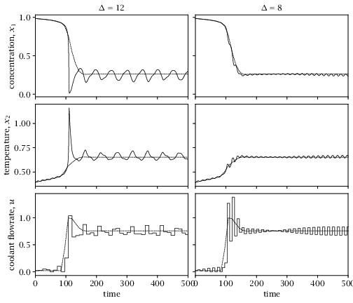
90 # [makes] tubempc_sampletimes.mat
## [rule] copymat
# [depends] functions/cstrparam.py
# [depends] functions/nominalmpc.py
# [depends] functions/tubempc.py
#
# Robust control of an exothermic reaction — effect of sample time.
# Note: takes ~3 min; the .mat is checked in to data/.
# If you change anything, re-run and copy tubempc_sampletimes.mat to data/.
import sys
import os
sys.path.insert(0, os.path.join(os.path.dirname(os.path.abspath(__file__)), 'functions'))

import numpy as np
from scipy.io import savemat
from scipy.interpolate import interp1d
from cstrparam import cstrparam
from nominalmpc import nominalmpc
from tubempc import tubempc


def resample_nominal(reftraj, Delta):
    """Resample the reference (central path) trajectory to a new sample time."""
    t = reftraj['t']
    u = reftraj['u']   # (Nu, Nsim_nom)
    x = reftraj['x']   # (Nx, Nsim_nom+1)

    t0, tf = t[0], t[-1]
    tnew = np.arange(t0, tf + 1e-10, Delta)

    # Interpolate u (defined at t[:-1]) and x (defined at t).
    u_interp = interp1d(t[:-1], u, kind='cubic', fill_value='extrapolate')
    x_interp = interp1d(t,      x, kind='cubic', fill_value='extrapolate')

    unew = u_interp(tnew)   # (Nu, len(tnew))
    xnew = x_interp(tnew)   # (Nx, len(tnew))

    return {'t': tnew, 'u': unew, 'x': xnew}


# Base parameters.
nompars = cstrparam()
nompars['tfinal']     = 600
nompars['colloc']     = 10
nompars['plantSteps'] = 20
nompars['A']          = 0.002
nompars['w']          = 0.4

# Two sample times.
Deltas = [8, 12]
predHorizon = 360
pars = {}
for Delta in Deltas:
    key = f'd{Delta}'
    pars[key] = nompars.copy()
    pars[key]['Delta'] = Delta
    pars[key]['N']     = round(predHorizon / Delta)
pars['d12']['colloc'] = 24   # More collocation points for longer interval.

# Run nominal (central path) MPC using Delta=12, then resample for Delta=8.
print('Running nominalmpc with Delta=12...')
reftraj = nominalmpc(pars['d12'])
pars['d12']['reftraj'] = reftraj
pars['d8']['reftraj']  = resample_nominal(reftraj, pars['d8']['Delta'])

# Run tube-based MPC for each sample time.
results = {}
for key in [f'd{d}' for d in Deltas]:
    print(f'Running tubempc for {key}...')
    results[key] = tubempc(pars[key])

# Build output data structure.
data = {}
data['ref'] = {
    'x1': reftraj['x'][0, :],
    'x2': reftraj['x'][1, :],
    'u':  reftraj['u'].flatten(),
    't':  reftraj['t'],
}
for key in [f'd{d}' for d in Deltas]:
    r = results[key]
    data[key] = {
        'x1':      r['x'][0, :],
        'x2':      r['x'][1, :],
        'x1plant': r['xplant'][0, :],
        'x2plant': r['xplant'][1, :],
        'u':       r['u'].flatten(),
        't':       r['t'],
        'tplant':  r['tplant'],
    }