Figure 3.9:

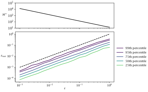
Observed probability \varepsilon _test of constraint violation for i=10. Distribution is based on 500 trials for each value of \varepsilon . Dashed line shows the outcome predicted by formula (3.25), i.e., \varepsilon _test = \varepsilon .

Code for Figure 3.9

Text of the GNU GPL.

main.m

 1
 2
 3
 4
 5
 6
 7
 8
 9
10
11
12
13
14
15
16
17
18
19
20
21
22
23
24
25
26
27
28
29
30
31
32
33
34
35
36
37
38
39
40
41
42
43
44
45
46
47
48
49
50
51
52
53
54
55
56
57
58
59
60
61
62
63
64
65
66
67
68
69
70
71
72
73
74
75
76
77
% Stochastic constraint tightening for a scalar system.



A = 1;
B = 1;
Q = 0.5;
R = 1;

K = -dlqr(A, B, Q, R);
AK = A + B*K;

U = [-1, 1];
X = [-1, 1];
W = [-0.5, 0.5];

N = 10; % Number of time points over which to consider disturbance.

SKinf = W/(1 - AK);
Ubar = U - abs(K)*SKinf;
Xbar_robust = X - SKinf;

% Helper function for state evolution matrix.

E = evolution(AK, 1, N); % Converts from vector of w(k) to vector of e(k).
rand('state', 0);
sampleE = @(n) E*(W(1) + (W(2) - W(1))*rand(N, n));

Ntrials = 500; % How many times to perform the constraint tightening.
beta = 0.01;
epsilons = logspace(-3, 0, 16);
Ms = ceil(2./epsilons*(2 - log(beta)));

esim = sampleE(1000000); % Number of simulations to calculate epsilon_test.

Xbar = NaN(2, length(Ms), Ntrials);
eviolation = NaN(length(Ms), Ntrials); % Holds samples of epsilon_test.
for i = 1:length(Ms)
    fprintf('%2d. epsilon = %10g (M = %d)\n', i, epsilons(i), Ms(i));
    for j = 1:Ntrials
        % Sample e sequence.
        e = sampleE(Ms(i));

        % Find min/max of e and check constraint violation.
        emin = min([e(1,:), 0]);
        emax = max([e(1,:), 0]);
        eviolation(i, j) = mean(esim(1,:) < emin) + mean(esim(1,:) > emax);

        % Tighten constraints on x.
        Xbar(1, i, j) = min(X(1) - emin, 0);
        Xbar(2, i, j) = max(X(2) - emax, 0);
    end
end


% Plot tightened sets.
labels = {'Xbar_{lb}', 'Xbar_{ub}'};
locations = {'SouthWest', 'NorthWest'};
for i = 1:2
    dum = violationquantiles(epsilons, Xbar(i,:,:), false());
    plot(epsilons([1, end]), Xbar_robust(i)*[1, 1], '-k', ...
         'DisplayName', 'Robust');
    xlabel('\epsilon');
    ylabel(labels{i});
    legend('location', locations{i});
    title('Tightened Constraints');
    axis([min(epsilons), max(epsilons), i - 2.1, i - 0.9]);
end

% Plot violation probabilities.
q = violationquantiles(epsilons, eviolation, true());
plot(epsilons, epsilons, '--k');
legend('off');
legend('location', 'SouthEast');
ylabel('\epsilon_{test}');
xlabel('\epsilon');
axis([min(epsilons), max(epsilons), 1e-6, 1]);

evolution.m

 1
 2
 3
 4
 5
 6
 7
 8
 9
10
11
12
13
14
function E = evolution(A, B, Nt)
    % Computes the state evolution matrix for N steps.
    [Nx, Nu] = size(B);
    E = zeros(Nt*Nx, Nt*Nu);
    e = [B, zeros(Nx, (Nt - 1)*Nu)];
    for k = 1:Nt
        i = ((k - 1)*Nx + 1):(k*Nx);
        E(i,:) = e;
        if k < Nt
            e = A*e;
            j = (k*Nu + 1):((k + 1)*Nu);
            e(:,j) = B;
        end
    end

violationquantiles.m

 1
 2
 3
 4
 5
 6
 7
 8
 9
10
11
12
13
14
15
16
17
18
19
20
21
22
function q = violationquantiles(x, v, logscale)
    % Plots quantiles of violation probability.
    narginchk(2, 3);
    if nargin() < 3
        logscale = true();
    end

    quantiles = [0.05, 0.25, 0.5, 0.75, 0.95];
    colors = jet(length(quantiles));
    q = quantile(squeeze(v), quantiles, 2);
    if logscale
        q = max(q, 1e-16);
        plotfunc = @loglog;
    else
        plotfunc = @semilogx;
    end
    figure();
    hold('on')
    for j = 1:length(quantiles)
        plotfunc(x, q(:,j), '-o', 'color', colors(j,:), ...
                 'DisplayName', sprintf('percentile %.0f', 100*quantiles(j)));
    end