Figure 4.5

Figure 4.5:

Evolution of the state (solid line) and MHE state estimate (dashed line).

Code for Figure 4.5

batchreactor.py


  1
  2
  3
  4
  5
  6
  7
  8
  9
 10
 11
 12
 13
 14
 15
 16
 17
 18
 19
 20
 21
 22
 23
 24
 25
 26
 27
 28
 29
 30
 31
 32
 33
 34
 35
 36
 37
 38
 39
 40
 41
 42
 43
 44
 45
 46
 47
 48
 49
 50
 51
 52
 53
 54
 55
 56
 57
 58
 59
 60
 61
 62
 63
 64
 65
 66
 67
 68
 69
 70
 71
 72
 73
 74
 75
 76
 77
 78
 79
 80
 81
 82
 83
 84
 85
 86
 87
 88
 89
 90
 91
 92
 93
 94
 95
 96
 97
 98
 99
100
101
102
103
104
105
106
107
108
109
110
111
112
113
114
115
116
117
118
119
120
121
122
123
124
125
126
127
128
129
130
131
132
133
134
135
136
137
138
139
140
141
142
143
144
145
146
147
148
149
150
151
152
153
154
155
156
157
158
159
160
161
162
163
164
165
166
167
168
169
170
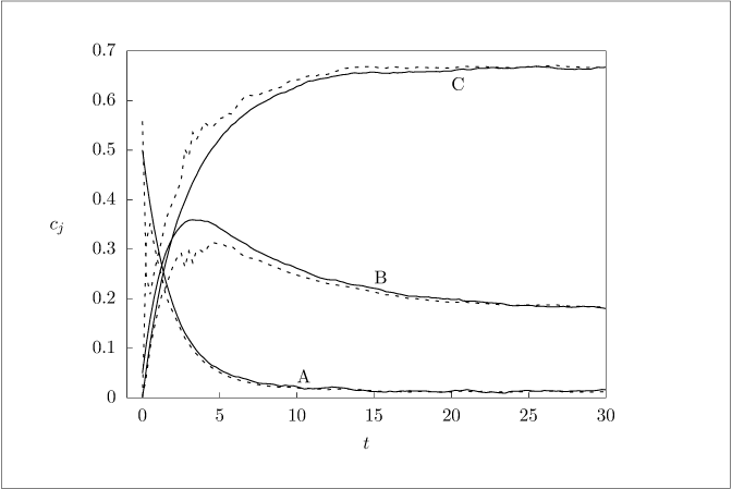
171 # pars = batchreactor(Nsim)
#
# Returns a struct of batch reactor parameters to avoid duplication across
# MHE, EKF, and UKF scripts.
import os
import numpy as np
import scipy.io
import matplotlib.pyplot as plt
import casadi
import mpctools

def batchreactor(Nsim):
    """
    pars = batchreactor(Nsim)

    Returns a struct of batch reactor parameters to avoid duplication across
    MHE, EKF, and UKF scripts.
    """
    if not isinstance(Nsim, int):
        raise TypeError("Nsim must be an integer")

    # Sizes
    Delta = 0.25
    Nx = 3
    Ny = 1
    Nw = Nx
    Nv = Ny

    # Random variable standard deviations
    sig_v = 0.25  # Measurement noise
    sig_w = 0.001 # State noise
    sig_p = 0.5   # Prior

    P = sig_p**2 * np.eye(Nx)
    Q = sig_w**2 * np.eye(Nw)
    R = sig_v**2 * np.eye(Ny)

    # Create symbolic variables
    x_sym = casadi.SX.sym('x', Nx)

    # Define ODE system
    ode = {'x': x_sym, 'ode': batch_model(x_sym)}

    # Create integrator
    plant = casadi.integrator('integrator', 'cvodes', ode, 0, Delta)

    # Create RK4 discretization with M=4 substeps to match MATLAB (getCasadiFunc M=4)
    frk4 = mpctools.getCasadiFunc(batch_model, [Nx], ['x'],
                                   funcname='frk4', rk4=True, Delta=Delta, M=4)

    # Create state transition and measurement functions
    w_sym = casadi.SX.sym('w', Nw)
    f = casadi.Function('f', [x_sym, w_sym], [frk4(x_sym) + w_sym], ['x', 'w'], ['f'])
    h = casadi.Function('h', [x_sym], [measurement(x_sym)], ['x'], ['h'])

    # Choose prior
    xhat0 = np.array([1.0, 0.0, 4.0])
    x0 = np.array([0.5, 0.05, 0.0])

    # Simulate system to get data
    np.random.seed(0)
    w = sig_w * np.random.randn(Nw, Nsim)
    v = sig_v * np.random.randn(Nv, Nsim + 1)

    xsim = np.nan * np.ones((Nx, Nsim + 1))
    xsim[:,0] = x0

    ysim = np.nan * np.ones((Ny, Nsim + 1))
    yclean = np.nan * np.ones((Ny, Nsim + 1))

    for t in range(Nsim + 1):
        xsim[:,t] = np.maximum(xsim[:,t], 0)
        yclean[:,t] = np.array(h(xsim[:,t])).flatten()
        ysim[:,t] = yclean[:,t] + v[:,t]

        if t < Nsim:
            xsim[:,t+1] = np.array(plant(x0=xsim[:,t])['xf']).flatten() + w[:,t]

    t = np.arange(Nsim + 1) * Delta

    # Package everything up
    pars = {
        'Delta': Delta,
        'Nsim': Nsim,
        'Nx': Nx,
        'Ny': Ny,
        'Nw': Nw,
        'Nv': Nv,
        'sig_v': sig_v,
        'sig_w': sig_w,
        'sig_p': sig_p,
        'P': P,
        'Q': Q,
        'R': R,
        'plant': plant,
        'frk4': frk4,
        'f': f,
        'h': h,
        'xhat0': xhat0,
        'x0': x0,
        'xsim': xsim,
        'ysim': ysim,
        'yclean': yclean,
        't': t,
        'reactorplot': reactorplot
    }

    return pars

def batch_model(x):
    """Nonlinear ODE function"""
    k1 = 0.5
    km1 = 0.05
    k2 = 0.2
    km2 = 0.01

    cA = x[0]
    cB = x[1]
    cC = x[2]

    rate1 = k1*cA - km1*cB*cC
    rate2 = k2*cB**2 - km2*cC

    return casadi.vertcat(
        -rate1,
        rate1 - 2*rate2,
        rate1 + rate2
    )

def measurement(x):
    """Linear measurement function"""
    RT = 0.0821 * 400
    return RT * casadi.sum1(x)

def reactorplot(x, xhat, y, yhat, yclean, Delta):
    """Make a plot of actual and estimated states"""
    if not all(isinstance(arg, np.ndarray) for arg in [x, xhat, y, yhat, yclean]):
        raise TypeError("Arrays must be numpy arrays")
    if not isinstance(Delta, (int, float)):
        raise TypeError("Delta must be numeric")
    if os.getenv('OMIT_PLOTS') == 'true':
        return None

    fig = plt.figure()
    Nx = 3
    Nt = x.shape[1] - 1
    t = np.arange(Nt + 1) * Delta

    plt.subplot(2, 1, 2)
    plt.plot(t, yclean, '-k', label='Actual')
    plt.plot(t, yclean, '--c', label='Measured')
    plt.plot(t, yhat, 'ok', label='Estimated')
    plt.ylabel('P')
    plt.xlabel('t')
    plt.legend(loc='center left', bbox_to_anchor=(1, 0.5))
    plt.ylim([10, 35])

    plt.subplot(2, 1, 1)
    colors = ['r', 'b', 'g']
    names = ['A', 'B', 'C']
    for i in range(Nx):
        plt.plot(t, x[i,:] + 1e-10, '-'+colors[i],
                label=f'Actual C_{names[i]}')
        plt.plot(t, xhat[i,:] + 1e-10, 'o'+colors[i],
                label=f'Estimated C_{names[i]}')
    plt.xlabel('t')
    plt.ylabel('c_i')
    plt.legend(loc='center left', bbox_to_anchor=(1, 0.5))
    plt.ylim([-1, 1.5])

    return fig

main.py


  1
  2
  3
  4
  5
  6
  7
  8
  9
 10
 11
 12
 13
 14
 15
 16
 17
 18
 19
 20
 21
 22
 23
 24
 25
 26
 27
 28
 29
 30
 31
 32
 33
 34
 35
 36
 37
 38
 39
 40
 41
 42
 43
 44
 45
 46
 47
 48
 49
 50
 51
 52
 53
 54
 55
 56
 57
 58
 59
 60
 61
 62
 63
 64
 65
 66
 67
 68
 69
 70
 71
 72
 73
 74
 75
 76
 77
 78
 79
 80
 81
 82
 83
 84
 85
 86
 87
 88
 89
 90
 91
 92
 93
 94
 95
 96
 97
 98
 99
100
101
102
103
104
105
106
107
108
109
110
111
112
113
114
115
116
117
118
119
120
121
122
123
124
125
126
127
128
129
130
131
132
133
134
135
136
137
138
139
140
141
142
143
144
145
146
147
148
149
150
151
152
153
154
155
156
157
158
159
160
161
162
163
164
165
166
167
168
169
170
171
172
173
174
175
176
177
178
179
180
181
182 # [makes] batchreactor_mhe.dat
# [depends] functions/batchreactor.py
#
# Simulates the Batch Reactor Example (3.2.1) from Haseltine & Rawlings (2005).
# MHE is implemented and it is shown that it performs better than EKF and UKF
# when a poor prior is used.
import sys
import os
sys.path.insert(0, os.path.join(os.path.dirname(os.path.abspath(__file__)), 'functions'))

import numpy as np
import scipy.linalg
import casadi
import mpctools as mpc
from misc import gnuplotsave
from batchreactor import batchreactor

Nsim = 120
pars = batchreactor(Nsim)
Nx   = pars['Nx']
Ny   = pars['Ny']
Nw   = pars['Nw']
Nv   = pars['Nv']
Nt   = 10
xsim = pars['xsim']
ysim = pars['ysim']

sig_w = pars['sig_w']
sig_v = pars['sig_v']

# Stage cost: w'w/sig_w^2 + v'v/sig_v^2
w_sym = casadi.SX.sym('w', Nw)
v_sym = casadi.SX.sym('v', Nv)
l = casadi.Function('l', [w_sym, v_sym],
                    [casadi.dot(w_sym, w_sym)/sig_w**2
                     + casadi.dot(v_sym, v_sym)/sig_v**2],
                    ['w', 'v'], ['l'])

# ── Smoothing prior support ──────────────────────────────────────────────────

# Jacobian functions for EKF step
x_jac = casadi.SX.sym('x_jac', Nx)
w_jac = casadi.SX.sym('w_jac', Nw)
f_jac = pars['f'](x_jac, w_jac)
A_fn    = casadi.Function('A_jac',   [x_jac, w_jac], [casadi.jacobian(f_jac, x_jac)])
Gdyn_fn = casadi.Function('Gdyn_jac',[x_jac, w_jac], [casadi.jacobian(f_jac, w_jac)])
C_fn    = casadi.Function('C_jac',   [x_jac],        [casadi.jacobian(pars['h'](x_jac), x_jac)])

# Shooting function from x[1] over Nt steps (Nt-1 [v,w] pairs, last meas has no v)
# W = [v[1];w[1]; v[2];w[2]; ...; v[Nt-1];w[Nt-1]]  shape (Nt-1)*(Nv+Nw)
x1_sh = casadi.SX.sym('x1', Nx)
W_sh  = casadi.SX.sym('W', (Nt - 1) * (Nv + Nw))
x_cur = x1_sh
y_sh  = []
idx   = 0
for k in range(Nt - 1):
    v_k   = W_sh[idx: idx + Nv];  idx += Nv
    w_k   = W_sh[idx: idx + Nw];  idx += Nw
    y_sh.append(pars['h'](x_cur) + v_k)
    x_cur = pars['f'](x_cur, w_k)
y_sh.append(pars['h'](x_cur))          # y[Nt]: no v[Nt] (matches Octave convention)
Y_sh = casadi.vertcat(*y_sh)            # shape (Nt*Ny,)
shoot_fn = casadi.Function('shoot', [x1_sh, W_sh],
                           [Y_sh,
                            casadi.jacobian(Y_sh, x1_sh),
                            casadi.jacobian(Y_sh, W_sh)],
                           ['x1', 'W'], ['Y', 'O', 'G'])

# Noise covariance block for Q_shoot = block_diag([R, Q_proc] * (Nt-1))
R_mat   = sig_v**2 * np.eye(Nv)
Q_proc  = sig_w**2 * np.eye(Nw)
Q_shoot = scipy.linalg.block_diag(
    *([scipy.linalg.block_diag(R_mat, Q_proc)] * (Nt - 1)))


def smoothing_update(solver, Pinv):
    """
    Returns (Pinv_new, x0bar_new) using the MHE smoothing prior update
    (matches Octave mpctools MHESolver.smoothingupdate).
    """
    xhat_0 = np.array(solver.var['x', 0]).flatten()
    xhat_1 = np.array(solver.var['x', 1]).flatten()

    # EKF step: measurement update at x[0], then predict to x[1]
    P      = np.linalg.inv(Pinv)
    xhatm  = np.array(pars['f'](xhat_0, np.zeros(Nw))).flatten()
    A      = np.array(A_fn(xhat_0,    np.zeros(Nw))).reshape(Nx, Nx)
    G_dyn  = np.array(Gdyn_fn(xhat_0, np.zeros(Nw))).reshape(Nx, Nw)
    C      = np.array(C_fn(xhat_0)).reshape(Ny, Nx)
    # H = I (additive measurement noise), so H*R*H' = R_mat
    S_ekf  = C @ P @ C.T + R_mat
    Pm     = (G_dyn @ Q_proc @ G_dyn.T
              + A @ P @ A.T
              - (A @ P @ C.T) @ np.linalg.solve(S_ekf, C @ P @ A.T))
    Pm     = 0.5 * (Pm + Pm.T)     # symmetrize

    # Shooting from xhatm (zero noise linearization point)
    W_zeros = np.zeros((Nt - 1) * (Nv + Nw))
    res     = shoot_fn(x1=xhatm, W=W_zeros)
    Y_bar   = np.array(res['Y']).flatten()                         # (Nt*Ny,)
    O_mat   = np.array(res['O']).reshape(Nt * Ny, Nx)             # (Nt*Ny, Nx)
    G_mat   = np.array(res['G']).reshape(Nt * Ny, (Nt-1)*(Nv+Nw))# (Nt*Ny, ...)

    # Actual measurements y[1..Nt] from solver (skip oldest y[0])
    Y = np.concatenate([np.array(solver.par['y', k]).flatten()
                        for k in range(1, Nt + 1)])
    E = Y - Y_bar

    # Innovation covariance from noise only (Pyx = G Q G')
    Pyx = G_mat @ Q_shoot @ G_mat.T
    Pyx += 1e-10 * np.eye(Nt * Ny)  # numerical regularization

    # Pinv_new = Pm^{-1}  (by Woodbury: Pxy^{-1} - O' Pyx^{-1} O = Pm^{-1})
    Pinv_new  = np.linalg.inv(Pm)
    Pinv_new  = 0.5 * (Pinv_new + Pinv_new.T)

    # x0bar_new = xhat[1] + Pm O' Pyx^{-1} (O (xhat[1] - xhatm) - E)
    x0bar_new = xhat_1 + Pm @ O_mat.T @ np.linalg.solve(Pyx, O_mat @ (xhat_1 - xhatm) - E)

    return Pinv_new, x0bar_new

# ── Prior cost: (x - x0bar)' Pinv (x - x0bar), with Pinv as a solver parameter ─

x_lx  = casadi.SX.sym('x_lx',   Nx)
xb_lx = casadi.SX.sym('x0bar_lx', Nx)
Pf_lx = casadi.SX.sym('Pinv_flat', Nx * Nx)
dx_lx = x_lx - xb_lx
lx = casadi.Function('lx', [x_lx, xb_lx, Pf_lx],
                     [casadi.mtimes(dx_lx.T,
                                    casadi.mtimes(casadi.reshape(Pf_lx, Nx, Nx),
                                                  dx_lx))],
                     ['x', 'x0bar', 'Pinv_flat'], ['lx'])

Pinv  = np.linalg.inv(pars['P'])
x0bar = pars['xhat0'].copy()

N  = {'x': Nx, 'w': Nw, 'y': Ny, 't': Nt}
lb = {'x': np.zeros((Nt + 1, Nx))}
ub = {'x': 10 * np.ones((Nt + 1, Nx))}

# y is TIME-FIRST: shape (Nt+1, Ny).  Load first full window of real data.
y_init = ysim[:, :Nt + 1].T.copy()   # (Nt+1, Ny)

solver = mpc.nmhe(pars['f'], pars['h'], np.zeros((Nt, 0)), y_init,
                  l, N, lx=lx, x0bar=x0bar,
                  lb=lb, ub=ub,
                  funcargs={'f': ['x', 'w'], 'h': ['x'], 'l': ['w', 'v'],
                            'lx': ['x', 'x0bar', 'Pinv_flat']},
                  par={'Pinv_flat': Pinv.ravel(order='F')},
                  verbosity=0)

xhat = np.full((Nx, Nsim + 1), np.nan)
yhat = np.full((Ny, Nsim + 1), np.nan)

for t in range(Nsim + 1):
    if t <= Nt:
        # Build up horizon: pad early slots with first available measurement.
        for k in range(Nt + 1):
            solver.par['y', k] = ysim[:, max(0, t - Nt + k)]
    else:
        solver.newmeasurement(ysim[:, t])

    status = solver.solve()
    if solver.stats['status'] != 'Solve_Succeeded':
        print('Warning: Solver failure at time %d!' % t)
        break

    solver.saveguess(toffset=1)
    xhat[:, t] = np.array(solver.var['x', Nt]).flatten()
    yhat[:, t] = np.array(pars['h'](xhat[:, t])).flatten()

    if t >= Nt:
        # Smoothing prior update (horizon full).
        Pinv, x0bar = smoothing_update(solver, Pinv)
        solver.par['x0bar',     0] = x0bar
        solver.par['Pinv_flat', 0] = Pinv.ravel(order='F')
    else:
        # Horizon still growing: just advance x0bar, keep initial Pinv.
        solver.par['x0bar', 0] = np.array(solver.var['x', 1]).flatten()

data_table = np.column_stack([pars['t'], xsim.T, xhat.T, ysim.T, yhat.T])
gnuplotsave('batchreactor_mhe.dat', data_table)