# sys = nonlinsys()#importnumpyasnpfromscipy.linalgimportsolve_discrete_arefromcontrolimportdlqrimportcasadidefnonlinsys():""" Returns a dict of parameters for the unstable nonlinear system. """# Initialize system dictsys={}# Define the model and stage costsys['Nx']=2sys['Nu']=2deff(x,u):returnnp.array([x[0]**2+x[1]+u[0]**3+u[1],x[0]+x[1]**2+u[0]+u[1]**3])sys['f']=fdefl(x,u):return0.5*(x.T@x+u.T@u)sys['l']=l# Define steady state and boundssys['xs']=np.zeros(sys['Nx'])sys['us']=np.zeros(sys['Nu'])sys['ulb']=np.array([-2.5,-2.5])sys['uub']=np.array([2.5,2.5])# Linearize the ODEx=casadi.SX.sym('x',sys['Nx'])u=casadi.SX.sym('u',sys['Nu'])f_expr=casadi.vertcat(x[0]**2+x[1]+u[0]**3+u[1],x[0]+x[1]**2+u[0]+u[1]**3)fcasadi=casadi.Function('f',[x,u],[f_expr])# Get JacobiansA=casadi.jacobian(f_expr,x)B=casadi.jacobian(f_expr,u)# Create functions to evaluate JacobiansA_func=casadi.Function('A',[x,u],[A])B_func=casadi.Function('B',[x,u],[B])# Evaluate at steady statesys['A']=np.array(A_func(sys['xs'],sys['us']))sys['B']=np.array(B_func(sys['xs'],sys['us']))# Linearize the objectivel_expr=0.5*(x.T@x+u.T@u)lcasadi=casadi.Function('l',[x,u],[l_expr])# Get HessiansQ=casadi.hessian(l_expr,x)[0]R=casadi.hessian(l_expr,u)[0]# Create functions to evaluate HessiansQ_func=casadi.Function('Q',[x,u],[Q])R_func=casadi.Function('R',[x,u],[R])sys['Q']=np.array(Q_func(sys['xs'],sys['us']))sys['R']=np.array(R_func(sys['xs'],sys['us']))# Compute LQR controllerK,S,E=dlqr(sys['A'],sys['B'],sys['Q'],sys['R'])sys['K']=-Ksys['P']=SdefVf(x):return0.5*x.T@sys['P']@xsys['Vf']=Vfreturnsys
# [ustar, uiter] = distributedgradient(V, u0, ulb, uub, ...)## Runs a distributed gradient algorithm for a problem with box constraints.## V should be a function handle defining the objective function. u0 should be# the starting point. ulb and uub should give the box constraints for u.## Additional arguments are passed as 'key' value pairs. They are as follows:## - 'beta', 'sigma' : parameters for line search (default 0.8 and 0.01)# - 'alphamax' : maximum step to take in any iteration (default 10)# - 'Niter' : Maximum number of iterations (default 25)# - 'steptol', 'gradtol' : Absolute tolerances on stepsize and gradient.# Algorithm terminates if the stepsize is less than# steptol and the gradient is less than gradtol# (defaults 1e-5 and 1e-6). Set either to a negative# value to never stop early.# - 'Nlinesearch' : maximum number of backtracking steps (default 100)# - 'I' : cell array defining the variables for each system. Default is# each variable is a separate system.## Return values are ustar, the final point, and uiter, a matrix of iteration# progress.importnumpyasnpfromcasadiimportSX,jacobian,Functiondefdistributedgradient(V,u0,ulb,uub,**kwargs):""" Runs a distributed gradient algorithm for a problem with box constraints. """# Get optionsparam={'beta':0.8,'sigma':0.01,'alphamax':15,'Niter':50,'steptol':1e-5,'gradtol':1e-6,'Nlinesearch':100,'I':None}param.update(kwargs)Nu=len(u0)ifparam['I']isNone:param['I']=[[i]foriinrange(Nu)]# Project initial condition to feasible spaceu0=np.minimum(np.maximum(u0,ulb),uub)# Get gradient function via CasADiusym=SX.sym('u',Nu)vsym=V(usym)Jsym=jacobian(vsym,usym)dVcasadi=Function('V',[usym],[Jsym])# Start the loopk=0uiter=np.full((Nu,param['Niter']+1),np.nan)uiter[:,0]=u0g,gred=calcgrad(dVcasadi,u0,ulb,uub)v=np.full(Nu,np.inf)whilek<param['Niter']and(np.linalg.norm(gred)>param['gradtol']ornp.linalg.norm(v)>param['steptol']):# Take stepuiter[:,k+1],v=coopstep(param['I'],V,g,uiter[:,k],ulb,uub,param)k+=1# Update gradientg,gred=calcgrad(dVcasadi,uiter[:,k],ulb,uub)# Get final point and strip off extra pointsuiter=uiter[:,:k+1]ustar=uiter[:,-1]returnustar,uiterdefcoopstep(I,V,g,u0,ulb,uub,param):""" Takes one step of cooperative distributed gradient projection. """Nu=len(u0)Ni=len(I)us=np.full((Nu,Ni),np.nan)Vs=np.full(Ni,np.nan)# Run each optimizationV0=float(V(u0))forjinrange(Ni):# Compute stepv=np.zeros(Nu)i=I[j]v[i]=-g[i]ubar=np.minimum(np.maximum(u0+v,ulb),uub)v=ubar-u0# Choose alphaifnp.any(ubar==ulb)ornp.any(ubar==uub):alpha=1.0else:withnp.errstate(divide='ignore'):alpha_lb=(ulb[i]-u0[i])/v[i]alpha_ub=(uub[i]-u0[i])/v[i]alpha=np.concatenate([alpha_lb,alpha_ub])alpha=alpha[np.isfinite(alpha)&(alpha>=0)]iflen(alpha)==0:alpha=0.0else:alpha=min(np.min(alpha),param['alphamax'])# Backtracking line searchk=1whilefloat(V(u0+alpha*v))>V0+param['sigma']*alpha*np.dot(g[i].flatten(),v[i].flatten()) \
andk<=param['Nlinesearch']:alpha=param['beta']*alphak+=1us[:,j]=u0+alpha*vVs[j]=float(V(us[:,j]))# Choose step to takew=np.ones(Ni)/Niforjinrange(Ni):# Check for descentu=us@wiffloat(V(u))<=np.dot(Vs,w):breakelifj==Ni-1:u=u0.copy()print('Warning: No descent directions!')break# Get rid of worst playerjmax=np.argmax(Vs)Vs[jmax]=-np.finfo(float).maxw[jmax]=0w=w/np.sum(w)# Calculate actual stepv=u-u0returnu,vdefcalcgrad(dV,u,ulb,uub):""" Calculates gradient and reduced gradient at a given point. """g=np.array(dV(u)).flatten()gred=g.copy()gred[(u==ulb)&(g>0)]=0gred[(u==uub)&(g<0)]=0returng,gred
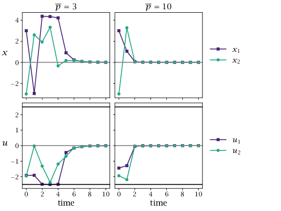
# Closed-loop evolution of nonlinear system for N = 2.# [depends] functions/nonlinsys.py functions/distributedgradient.py# [makes] nonlinsys_cl.matimportsysimportosimportmatplotlib.pyplotaspltimportnumpyasnpimportcasadiascaimportscipy.ioassiosys.path.append('functions/')fromnonlinsysimportnonlinsysfromdistributedgradientimportdistributedgradientsys=nonlinsys()# CasADi-compatible dynamics and costs (sys['f']/sys['Vf'] use numpy internally).P=sys['P']deff_ca(x,u):returnca.vertcat(x[0]**2+x[1]+u[0]**3+u[1],x[0]+x[1]**2+u[0]+u[1]**3)defl_ca(x,u):return0.5*(x[0]**2+x[1]**2+u[0]**2+u[1]**2)defVf_ca(x):Px0=P[0,0]*x[0]+P[0,1]*x[1]Px1=P[1,0]*x[0]+P[1,1]*x[1]return0.5*(x[0]*Px0+x[1]*Px1)# Define objective function and bounds.Nt=2Nu=sys['Nu']Nx=sys['Nx']defmake_V(Nt,Nu):defV(x,u):returnVf_ca(x)fortinrange(Nt-1,-1,-1):i=slice(t*Nu,(t+1)*Nu)defV_new(x,u,i=i,V_prev=V):returnl_ca(x,u[i])+V_prev(f_ca(x,u[i]),u)V=V_newreturnVV=make_V(Nt,Nu)ulb=np.tile(sys['ulb'],Nt)uub=np.tile(sys['uub'],Nt)I=[list(range(i,Nt*Nu,Nu))foriinrange(Nu)]defwarmstart(x,u,model):"""Fills in a warm start using the terminal control law."""Nt=u.shape[1]x_full=np.hstack([x.reshape(-1,1),np.full((len(x),Nt),np.nan)])u=u.copy()fortinrange(Nt):ifnp.any(np.isnan(u[:,t])):u[:,t]=np.minimum(np.maximum(sys['K']@x_full[:,t],sys['ulb']),sys['uub'])ifmodel=='nonlinear':x_full[:,t+1]=np.array(sys['f'](x_full[:,t],u[:,t])).flatten()elifmodel=='linear':x_full[:,t+1]=sys['A']@x_full[:,t]+sys['B']@u[:,t]else:raiseValueError('Invalid choice for model!')returnx_full,u# Simulate closed loop for different numbers of iterations.Nsim=10Ps=[3,10]options={}options['p3']={'alphamax':50,'beta':0.95}x0=np.array([3.,-3.])data={}forP_valinPs:key=f'p{P_val}'opts=options.get(key,{})x=np.full((Nx,Nsim+1),np.nan)x[:,0]=x0u=np.full((Nu,Nsim),np.nan)# Generate initial guess using the linear control law._,uguess=warmstart(x0,np.full((Nu,Nt),np.nan),'linear')# Simulate in closed loop.fortinrange(Nsim):useq,_=distributedgradient(lambdau,xt=x[:,t]:V(xt,u),uguess.flatten(order='F'),ulb,uub,I=I,Niter=P_val,**opts)u[:,t]=useq[:Nu]x[:,t+1]=np.array(sys['f'](x[:,t],u[:,t])).flatten()uguess=np.hstack([useq[Nu:].reshape(Nu,Nt-1),np.full((Nu,1),np.nan)])_,uguess=warmstart(x[:,t+1],uguess,'nonlinear')ifnp.linalg.norm(x[:,t+1])>100:importwarningswarnings.warn('x has diverged!')breaktplot=np.arange(Nsim+1)ifnotos.getenv('OMIT_PLOTS')=='true':plt.figure()plt.subplot(2,1,1)plt.plot(tplot,x[0,:],'-or')plt.plot(tplot,x[1,:],'-sb')plt.title(f'p = {P_val}')plt.subplot(2,1,2)plt.step(tplot,np.append(u[0,:],u[0,-1]),'-or',where='post')plt.step(tplot,np.append(u[1,:],u[1,-1]),'-sb',where='post')plt.plot([0,Nsim],[ulb[0]]*2,':k',[0,Nsim],[uub[0]]*2,':k')data[key]={'t':tplot,'x':x,'u':u,'ulb':ulb,'uub':uub}