Figure 8.11:

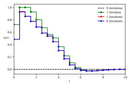
Gauss-Newton iterations for the direct multiple-shooting method

Code for Figure 8.11

Text of the GNU GPL.

main.m

 1
 2
 3
 4
 5
 6
 7
 8
 9
10
11
12
13
14
15
16
17
18
19
20
21
22
23
24
25
26
27
28
29
30
31
32
33
34
35
36
37
38
39
40
41
42
43
44
45
46
47
48
49
50
51
52
53
54
55
56
57
58
59
60
61
62
63
64
65
66
67
68
69
70
71
72
73
74
75
76
77
78
% Solves the minimization problem with T=10
%  minimize       1/2*integral{t=0 until t=T}(x1^2 + x2^2 + u^2) dt
%  subject to     dot(x1) = (1-x2^2)*x1 - x2 + u,   x1(0)=0, x1(T)=0
%                 dot(x2) = x1,                     x2(0)=1, x2(T)=0
%                 x1(t) >= -0.25, 0<=t<=T
% Joel Andersson, UW Madison 2017
%
% States and control
x1 = casadi.SX.sym('x1');
x2 = casadi.SX.sym('x2');
u = casadi.SX.sym('u');

% Model equations
x1_dot = (1-x2^2)*x1 - x2 + u;
x2_dot = x1;

% Least squares objective terms
lsq =[x1; x2; u];

% Define the problem structure
ocp = struct('x',[x1; x2],'u',u, 'ode', [x1_dot; x2_dot], 'lsq',lsq);

% Specify problem data
data = struct('T', 10,...
              'x0', [0;1],...
              'xN', [ 0; 0],...
              'x_min', [-0.25; -inf],...
              'x_max', [ inf;  inf],...
              'x_guess',  [0; 0],...
              'u_min', -1,...
              'u_max', 1,...
              'u_guess', 0);

% Specify solver options
opts = struct('N', 20,...
	      'verbose', false);

% Create an OCP solver instance
s = dms_gn(ocp, data, opts);

% Display sparsities
figure();
subplot(1,2,1);
spy(sparse(casadi.DM(s.nlp.J.sparsity(), 1)), '.')
title('J sparsity pattern:')
subplot(1,2,2);
spy(sparse(casadi.DM(s.nlp.H.sparsity(), 1)), '.')
title('H sparsity pattern:')

% Initializing figure
figure;
clf;
hold on;
grid on;

% Plot solution
x1_plot = plot(s.t, s.sol.x(1,:), 'r--');
x2_plot = plot(s.t, s.sol.x(2,:), 'b-');
u_plot = stairs(s.t, [s.sol.u(1,:) nan], 'g-.');

xlabel('t')
legend('x1','x2','u')
pause(2);

iter=0;
while s.sol.norm_dw > 1e-8
     % SQP iteration
     s.sqpstep();
     iter = iter + 1;


     % Update plots
     set(x1_plot, 'Ydata', s.sol.x(1, :));
     set(x2_plot, 'Ydata', s.sol.x(2, :));
     set(u_plot, 'Ydata', s.sol.u(1,:));
     title(sprintf('Iteration %d, |dw| = %g', iter, s.sol.norm_dw))
     pause(2);
end

dms_gn.m

  1
  2
  3
  4
  5
  6
  7
  8
  9
 10
 11
 12
 13
 14
 15
 16
 17
 18
 19
 20
 21
 22
 23
 24
 25
 26
 27
 28
 29
 30
 31
 32
 33
 34
 35
 36
 37
 38
 39
 40
 41
 42
 43
 44
 45
 46
 47
 48
 49
 50
 51
 52
 53
 54
 55
 56
 57
 58
 59
 60
 61
 62
 63
 64
 65
 66
 67
 68
 69
 70
 71
 72
 73
 74
 75
 76
 77
 78
 79
 80
 81
 82
 83
 84
 85
 86
 87
 88
 89
 90
 91
 92
 93
 94
 95
 96
 97
 98
 99
100
101
102
103
104
105
106
107
108
109
110
111
112
113
114
115
116
117
118
119
120
121
122
123
124
125
126
127
128
129
130
131
132
133
134
135
136
137
138
139
140
141
142
143
144
145
146
147
148
149
150
151
152
153
154
155
156
157
158
159
160
161
162
163
164
165
166
167
168
169
170
171
172
173
174
175
176
177
178
179
180
181
182
183
184
185
186
187
188
189
190
191
192
193
194
195
196
197
198
199
200
201
202
203
204
205
206
207
208
209
210
211
212
213
214
215
216
217
218
219
220
221
222
223
224
225
226
227
228
229
230
231
232
classdef dms_gn < handle
  properties
    % Symbolic representation of the OCP
    ocp
    % OCP data
    data
    % Solver options
    opts
    % Verbose output
    verbose
    % Dimensions
    N
    nx
    nu
    % Solution time grid
    t
    % Control interval length
    dt
    % CasADi function objects
    fun
    % Nonlinear program
    nlp
    % Current iteration
    n_iter
    % Current solution
    sol
  end
  methods
    function self = dms_gn(ocp, data, opts)
      % Constructor
      self.ocp = ocp;
      self.data = data;
      self.opts = opts;

      % Verbosity?
      if (isfield(opts, 'verbose'))
	self.verbose = opts.verbose;
      else
	self.verbose = true;
      end

      % Problem dimensions
      self.N = self.opts.N;
      self.nx = numel(self.ocp.x);
      self.nu = numel(self.ocp.u);

      % Time grid
      self.t = linspace(0, data.T, self.N+1);

      % Interval length
      self.dt = data.T / self.N;

      % Get discrete-time dynamics
      self.rk4();

      % Transcribe to NLP
      self.transcribe();

      % Initialize x
      self.sol.w = self.nlp.w0;

      % Extract x,u from w
      [x_traj,u_traj] = self.fun.traj(self.sol.w);
      self.sol.x = full(x_traj);
      self.sol.u = full(u_traj);

      % Initialize Gauss-Newton method
      self.init_gauss_newton();
    end

    function init_gauss_newton(self)
      % Linearize the problem w.r.t. w
      self.nlp.J = jacobian(self.nlp.g, self.nlp.w);
      self.nlp.JM = jacobian(self.nlp.M, self.nlp.w);

      % Gauss-Newton Hessian and gradient
      self.nlp.H = self.nlp.JM' * self.nlp.JM;
      self.nlp.c = self.nlp.JM' * self.nlp.M;

      % Functions for calculating g, J, H
      self.fun.g = casadi.Function('g', {self.nlp.w}, {self.nlp.g},...
                                   {'w'}, {'g'});
      self.fun.J = casadi.Function('J', {self.nlp.w}, {self.nlp.J},...
                                   {'w'}, {'J'});
      self.fun.H = casadi.Function('H', {self.nlp.w}, {self.nlp.H, self.nlp.c},...
                                   {'w'}, {'H', 'c'});

      % Out new step is determined by solving the quadratic program for
      % dw = w_new-w
      %        minimize    1/2 dw'*H*dw + c'*dw
      %        subject to  g + A*dw = 0
      %                    lbw-w <= dw <= ubw-w
      qp = struct('h', self.nlp.H.sparsity(), 'a', self.nlp.J.sparsity());
      qp_options = struct();
      if ~self.verbose
        qp_options.printLevel = 'none';
      end
      self.fun.qp_solver = casadi.conic('qp_solver', 'qpoases', qp, qp_options);

      % Iteration counter
      self.n_iter = 0;

      % Residual
      self.sol.norm_dw = inf;
    end

    function rk4(self)
        % Continuous-time dynamics
        x = self.ocp.x;
        u = self.ocp.u;
        ode = self.ocp.ode;
        f = casadi.Function('f', {x, u}, {ode}, {'x','p'}, {'ode'});

        % Implement RK4 integrator that takes a single step
        k1 = f(x, u);
        k2 = f(x+0.5*self.dt*k1, u);
        k3 = f(x+0.5*self.dt*k2, u);
        k4 = f(x+self.dt*k3, u);
        xk = x+self.dt/6.0*(k1+2*k2+2*k3+k4);

        % Return as a function
        self.fun.F = casadi.Function('RK4', {x,u}, {xk}, {'x0','p'}, {'xf'});

	% Least squares objective function
	lsq = self.ocp.lsq;
	self.fun.Lsq = casadi.Function('Lsq', {x, u}, {lsq}, {'x','p'}, {'lsq'});
    end

    function transcribe(self)
      % Start with an empty NLP
      w = {}; % Variables
      g = {}; % Equality constraints
      M = {}; % Least squares objective function
      lbw = {}; % Lower bound on w
      ubw = {}; % Upper bound on w
      w0 = {}; % Initial guess for w

      % Expressions corresponding to the trajectories we want to plot
      x_plot = {};
      u_plot = {};

      % Initial conditions
      xk = casadi.MX.sym('x0', self.nx);
      w{end+1} = xk;
      lbw{end+1} = self.data.x0;
      ubw{end+1} = self.data.x0;
      w0{end+1} = self.data.x_guess;
      x_plot{end+1} = xk;

      % Loop over all times
      for k=0:self.N-1
          % Define local control
          uk = casadi.MX.sym(['u' num2str(k)], self.nu);
          w{end+1} = uk;
          lbw{end+1} = self.data.u_min;
          ubw{end+1} = self.data.u_max;
          w0{end+1} = self.data.u_guess;
          u_plot{end+1} = uk;

          % Simulate the system forward in time
          Fk = self.fun.F('x0', xk, 'p', uk);
    	  x_next = Fk.xf;

          % Add least squares term to the objective
          M{end+1} = self.fun.Lsq(xk, uk);

          % Define state at the end of the interval
          xk = casadi.MX.sym(['x' num2str(k+1)], self.nx);
          w{end+1} = xk;
          if k==self.N-1
              lbw{end+1} = self.data.xN;
              ubw{end+1} = self.data.xN;
          else
              lbw{end+1} = self.data.x_min;
              ubw{end+1} = self.data.x_max;
          end
          w0{end+1} = self.data.x_guess;
          x_plot{end+1} = xk;

          % Impose continuity
          g{end+1} = xk - x_next;
      end

      % Concatenate variables and constraints
      self.nlp.w = vertcat(w{:});
      self.nlp.g = vertcat(g{:});
      self.nlp.M = vertcat(M{:});
      self.nlp.lbw = vertcat(lbw{:});
      self.nlp.ubw = vertcat(ubw{:});
      self.nlp.w0 = vertcat(w0{:});

      % Create a function that maps the NLP decision variable to the x and u trajectories
      self.fun.traj = casadi.Function('traj', {self.nlp.w}, {horzcat(x_plot{:}), horzcat(u_plot{:})},...
	                             {'w'}, {'x', 'u'});
    end

    function sqpstep(self)
      % Update iteration counter
      self.n_iter = self.n_iter + 1;

      % Calculate the QP matrices
      self.sol.g = self.fun.g(self.sol.w);
      self.sol.J = self.fun.J(self.sol.w);
      [self.sol.H, self.sol.c] = self.fun.H(self.sol.w);

      % Solve the QP to get the step in in w
      qp_solution = self.fun.qp_solver('a', self.sol.J, 'h', self.sol.H, 'g', self.sol.c,...
				       'lbx', self.nlp.lbw-self.sol.w,...
				       'ubx', self.nlp.ubw-self.sol.w,...
				       'lba', -self.sol.g, 'uba', -self.sol.g, 'x0', 0);
      dw = full(qp_solution.x);

      % Check convergence criteria
      self.sol.norm_dw = norm(dw);

      % Take (full) step
      self.sol.w = self.sol.w + dw;

      % Extract x,u from w
      [x_traj,u_traj] = self.fun.traj(self.sol.w);
      self.sol.x = full(x_traj);
      self.sol.u = full(u_traj);

      % Print progress
      if self.verbose || mod(self.n_iter,10)==1
        disp(repmat('-', 1, 70))
        fprintf('%15s %15s\n', 'SQP iteration', 'norm(dw)');
      end
      fprintf('%15d %15g\n', self.n_iter, self.sol.norm_dw);
    end
  end
end