Figure 8.2(b)

Figure 8.2(b):

Performance of different integration methods. Simulation results for M=32.

Code for Figure 8.2(b)

butcherintegration.py


  1
  2
  3
  4
  5
  6
  7
  8
  9
 10
 11
 12
 13
 14
 15
 16
 17
 18
 19
 20
 21
 22
 23
 24
 25
 26
 27
 28
 29
 30
 31
 32
 33
 34
 35
 36
 37
 38
 39
 40
 41
 42
 43
 44
 45
 46
 47
 48
 49
 50
 51
 52
 53
 54
 55
 56
 57
 58
 59
 60
 61
 62
 63
 64
 65
 66
 67
 68
 69
 70
 71
 72
 73
 74
 75
 76
 77
 78
 79
 80
 81
 82
 83
 84
 85
 86
 87
 88
 89
 90
 91
 92
 93
 94
 95
 96
 97
 98
 99
100
101
102
103
104
105
106
107
108
109
110
111
112
113
114
115
116
117
118
119
120
121
122
123 # [xplus, converged, iter, k] = butcherintegration(x, f, h, a, b, [Niter=100])
#
# Performs numerical integration of f starting from x for h time units.
#
# f must be a function handle that returns dx/dt. If a defines an implicit
# method, f may also return the Jacobian as a second output; if so, Newton's
# method is used. Otherwise, fixed-point iteration is used.
#
# a and b should be the coefficients from the Butcher tableau for the
# integration scheme. Scalars are accepted for 1-stage methods. If the a
# matrix is strictly lower triangular, the explicit formulas are used.
#
# Niter is the maximum number of iterations to perform.
import numpy as np
from numpy.linalg import norm
from scipy.linalg import solve

def butcherintegration(x, func, h, a, b, Niter=100):
    """
    Performs numerical integration of f starting from x for h time units.

    Returns (xplus, converged, iter, k).
    """
    x = np.asarray(x, dtype=float).reshape(-1)
    Nx = len(x)

    # Accept scalars for 1-stage methods.
    if np.isscalar(a):
        a = np.array([[a]], dtype=float)
    else:
        a = np.asarray(a, dtype=float)
    if np.isscalar(b):
        b = np.array([b], dtype=float)
    else:
        b = np.asarray(b, dtype=float)

    Ns = len(b)
    if a.shape != (Ns, Ns):
        raise ValueError('a must be square with one row/col per element of b!')

    b = h * b
    a = h * a

    if np.count_nonzero(np.triu(a)) == 0:
        k = _butcher_explicit(x, func, a)
        converged = True
        niter = 0
    else:
        # Probe whether func returns a Jacobian.
        test = func(x)
        has_jac = isinstance(test, tuple)
        if has_jac:
            k, converged, niter = _butcher_implicit_newton(x, func, a, Niter)
        else:
            k, converged, niter = _butcher_implicit_fixedpoint(x, func, a, Niter)

    xplus = x + k @ b
    return xplus, converged, niter, k


def _butcher_explicit(x, func, a):
    """Explicit integration step."""
    Nx = len(x)
    Ns = a.shape[0]
    k = np.zeros((Nx, Ns))
    for i in range(Ns):
        val = func(x + k @ a[i, :])
        k[:, i] = np.asarray(val).reshape(-1)
    return k


def _butcher_implicit_newton(x, func, a, Niter):
    """Implicit step via Newton's method (func must return (f, J))."""
    Nx = len(x)
    Ns = a.shape[0]
    k = np.zeros((Nx, Ns))
    converged = False
    niter = 0

    while not converged and niter < Niter:
        niter += 1
        dX = k @ a.T
        if Ns == 1:
            f, J = func(x + dX.reshape(-1))
            f = np.asarray(f).reshape(-1)
            J = np.asarray(J) * a[0, 0]
        else:
            f = np.zeros(Nx * Ns)
            J = np.zeros((Nx * Ns, Nx * Ns))
            for i in range(Ns):
                I = slice(i * Nx, (i + 1) * Nx)
                fi, Ji = func(x + dX[:, i])
                f[I] = np.asarray(fi).reshape(-1)
                J[I, :] = np.kron(a[i, :], np.asarray(Ji))

        f = f - k.flatten(order='F')
        J = J - np.eye(Nx * Ns)
        dk = -solve(J, f)
        k = k + dk.reshape(Nx, Ns, order='F')
        converged = norm(dk) < 1e-8

    return k, converged, niter


def _butcher_implicit_fixedpoint(x, func, a, Niter):
    """Implicit step via fixed-point iteration (func returns only f)."""
    Nx = len(x)
    Ns = a.shape[0]
    k = np.zeros((Nx, Ns))
    converged = False
    niter = 0

    while not converged and niter < Niter:
        niter += 1
        k_old = k.copy()
        dX = k @ a.T
        for i in range(Ns):
            xi = (x + dX[:, i]) if Ns > 1 else (x + dX.reshape(-1))
            val = func(xi)
            k[:, i] = np.asarray(val).reshape(-1)
        converged = norm(k - k_old) < 1e-10

    return k, converged, niter

errorplot2d.py


 1
 2
 3
 4
 5
 6
 7
 8
 9
10
11
12
13
14
15
16
17
18
19
20
21
22
23
24
25
26
27
28 # errorplot2d(x, T, [location])
#
# Makes a phase plot of 2D trajectories. x is a dict mapping names to (2, N)
# arrays. If x contains an 'exact' key it is plotted as a solid black line;
# all others are plotted as dashed lines.
import os
import matplotlib.pyplot as plt

def errorplot2d(x, T, location=None):
    if os.getenv('OMIT_PLOTS') == 'true':
        return
    """
    Makes a phase plot of 2D trajectories.

    x must be a dict with string keys mapping to (2, N) arrays. The 'exact'
    key, if present, is plotted as a solid black line; others as dashed.
    """
    plt.figure()
    for key in x:
        style = '-k' if key == 'exact' else '--'
        plt.plot(x[key][0, :], x[key][1, :], style, label=key)
    plt.axis('equal')
    if location:
        plt.legend(loc=location)
    else:
        plt.legend()
    plt.xlabel('$x_1$')
    plt.ylabel('$x_2$', rotation=0)

main.py


 1
 2
 3
 4
 5
 6
 7
 8
 9
10
11
12
13
14
15
16
17
18
19
20
21
22
23
24
25
26
27
28
29
30
31
32
33
34
35
36
37
38
39
40
41
42
43
44
45
46
47
48
49
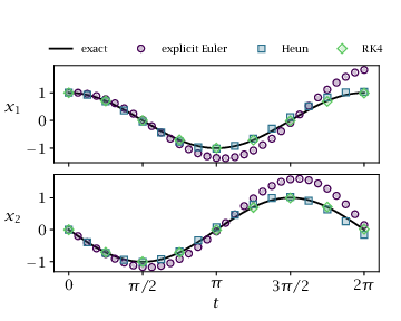
50 # Example explicit numerical integration of a linear ODE.
# [depends] functions/butcherintegration.py functions/errorplot2d.py
# [makes] explicitint_example.mat
import os
import sys
sys.path.insert(0, os.path.join(os.path.dirname(os.path.abspath(__file__)), 'functions'))

import numpy as np
import scipy.io
from butcherintegration import butcherintegration
from errorplot2d import errorplot2d

# Butcher tableaus
tabs = {}
tabs['euler'] = {'a': np.array([[0]]), 'b': np.array([1])}
tabs['heun'] = {'a': np.array([[0, 0], [1, 0]]), 'b': np.array([0.5, 0.5])}
tabs['rk4'] = {'a': np.array([[0, 0, 0, 0],
                             [0.5, 0, 0, 0],
                             [0, 0.5, 0, 0],
                             [0, 0, 1, 0]]),
               'b': np.array([1/6, 1/3, 1/3, 1/6])}
tabnames = list(tabs.keys())

# Run each method
A = np.array([[0, 1], [-1, 0]])
def f(x):
    return A @ x.reshape(-1,1)
x0 = np.array([[1], [0]])
T = 2*np.pi
Meval = 32
x = {}

for n in tabnames:
    Nstep = int(np.ceil(Meval/len(tabs[n]['b'])))
    h = T/Nstep
    x[n] = np.zeros((2, Nstep + 1))
    x[n][:,0] = x0.flatten()
    for i in range(Nstep):
        x[n][:,i+1], *_ = butcherintegration(x[n][:,i], f, h,
                                            tabs[n]['a'], tabs[n]['b'])

# Add exact solution
theta = np.linspace(0, 2*np.pi, 257)
x['exact'] = np.vstack((np.cos(theta), -np.sin(theta)))

# Make plot
errorplot2d(x, T, 'lower right')

# Save data
scipy.io.savemat('explicitint_example.mat', {'x': x, 'T': T})