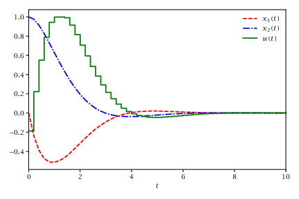
# [makes] single_shooting.mat# Solves the following minimization problem using direct single shooting# minimize 1/2*integral{t=0 until t=T}(x1^2 + x2^2 + u^2) dt# subject to dot(x1) = (1-x2^2)*x1 - x2 + u, x1(0)=0, x1(T)=0# dot(x2) = x1, x2(0)=1, x2(T)=0# with T=10## This example can be found in CasADi's example collection in MATLAB/Octave,# Python and C++ formats.## Joel Andersson, UW Madison 2017importnumpyasnpimportcasadifromscipy.ioimportsavemat# States and controlx1=casadi.SX.sym('x1')x2=casadi.SX.sym('x2')u=casadi.SX.sym('u')# Model equationsx1_dot=(1-x2**2)*x1-x2+ux2_dot=x1# Objective function (integral term)quad=x1**2+x2**2+u**2# Problem structureocp=dict(x=casadi.vertcat(x1,x2),u=u,ode=casadi.vertcat(x1_dot,x2_dot),quad=quad)# Problem datadata=dict(T=10.0,x0=np.array([0.0,1.0]),xN=np.array([0.0,0.0]),u_min=-1.0,u_max=1.0,u_guess=0.0)# Solver optionsopts=dict(N=50,verbose=True)# Problem independent code from here on# Problem dimensionsN=opts['N']nx=ocp['x'].numel()nu=ocp['u'].numel()# Time gridtgrid=np.linspace(0,data['T'],N+1)# Continuous-time dynamics as a functionf=casadi.Function('f',[ocp['x'],ocp['u']],[ocp['ode'],ocp['quad']],['x','p'],['ode','quad'])# RK4 integrator that takes a single stepdt=data['T']/Nx0sym=casadi.MX.sym('x0',nx)psym=casadi.MX.sym('p',nu)k1,k1q=f(x0sym,psym)k2,k2q=f(x0sym+dt/2*k1,psym)k3,k3q=f(x0sym+dt/2*k2,psym)k4,k4q=f(x0sym+dt*k3,psym)xf=x0sym+dt*(k1+2*k2+2*k3+k4)/6qf=dt*(k1q+2*k2q+2*k3q+k4q)/6F=casadi.Function('RK4',[x0sym,psym],[xf,qf],['x0','p'],['xf','qf'])# Start with an empty NLPw=[]lbw=[]ubw=[]w0=[]g=[]J=0# Expressions corresponding to the trajectories we want to plotx_plot=[]u_plot=[]# Initial conditionsxk=casadi.DM(data['x0'])x_plot.append(xk)# Loop over all timesforkinrange(N):# Declare local controluk=casadi.MX.sym('u{}'.format(k),nu)w.append(uk)lbw.append(data['u_min'])ubw.append(data['u_max'])w0.append(data['u_guess'])u_plot.append(uk)# Simulate the system forward in timeFk=F(x0=xk,p=uk)# Add contribution to objective functionJ=J+Fk['qf']# Update xxk=Fk['xf']x_plot.append(xk)# Enforce terminal conditionsg.append(xk-data['xN'])# Concatenate variables and constraintsw=casadi.vertcat(*w)lbw=casadi.vertcat(*lbw)ubw=casadi.vertcat(*ubw)w0=casadi.vertcat(*w0)g=casadi.vertcat(*g)# Formulate the NLP solver objectnlp=dict(x=w,g=g,f=J)solver=casadi.nlpsol('solver','ipopt',nlp)# Create a function that maps the NLP decision variable to the x and u trajectoriestraj=casadi.Function('traj',[w],[casadi.horzcat(*x_plot),casadi.horzcat(*u_plot)],['w'],['x','u'])# Solve the NLP and extract solutionsol=solver(x0=w0,lbx=lbw,ubx=ubw,lbg=0,ubg=0)x_opt,u_opt=traj(sol['x'])x_opt=np.array(x_opt)u_opt=np.array(u_opt)savemat('single_shooting.mat',{'tgrid':tgrid,'x_opt':x_opt,'u_opt':u_opt})