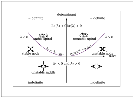
Figure 2.1:

Dynamical regimes for the planar system dx/dt = Ax, A \in \mathbb {R}^{2 x2}.

Code for Figure 2.1

Text of the GNU GPL.

main.m

  1
  2
  3
  4
  5
  6
  7
  8
  9
 10
 11
 12
 13
 14
 15
 16
 17
 18
 19
 20
 21
 22
 23
 24
 25
 26
 27
 28
 29
 30
 31
 32
 33
 34
 35
 36
 37
 38
 39
 40
 41
 42
 43
 44
 45
 46
 47
 48
 49
 50
 51
 52
 53
 54
 55
 56
 57
 58
 59
 60
 61
 62
 63
 64
 65
 66
 67
 68
 69
 70
 71
 72
 73
 74
 75
 76
 77
 78
 79
 80
 81
 82
 83
 84
 85
 86
 87
 88
 89
 90
 91
 92
 93
 94
 95
 96
 97
 98
 99
100
101
102
103
104
105
106
107
108
109
110
111
112
113
114
115
116
117
118
119
120
121
% the complicated planar dynamics figure()
% jbr, 9/25/2011

% axes and (trace)^2 = 4 det line

x = linspace(-5,5,101)';
y = x.*x/4;
quad = [x, y];
lines = [-5, 0, 0, -7,   0, -1.5; ...
          5, 0, 0, -2.5, 0,   10];

% stable spiral
T = -0.2;
D = (T^2+4)/4;
A = [0, sqrt(D); -sqrt(D), T];
nts = 101;
time = linspace(0,15,nts)';
x0 = [1;1];
x = zeros(2,nts);
for  i = 1:length(time);
  x(:,i) = expm(A*time(i))*x0;
end
xssp = x';


% put an arrow on the phase plot at the 11th point;
% size of arrow is adjusted by value of scale
nrow = 11;
s = "stable spiral";
% skip = 4;
% setarrow(s, nrow, skip, xssp)
s
xssp(nrow,:)


% unstable sprial; reverse time
%T = 0.2;
%D = (T^2+4)/4;
%A = [0, sqrt(D); -sqrt(D), T];
%x0 = [0.1;0.1];
x0 = [-1; -1];
x = zeros(2,nts);
for  i = 1:length(time);
  x(:,i) = expm(A*time(i))*x0;
end
xusp = x';
xusp = flipud(xusp);
% put an arrow on the phase plot 10 points from the end
nrow = size(xusp,1) - 10;
s = "unstable spiral";
% skip = 4;
% setarrow(s, nrow, skip, xusp);
s
xusp(nrow,:)


% stable node
% T = -1 + -0.5;
% D = (-1)*(-0.5);
A = [-0.5, 0; 0, -0.25];
x0 = [1;1];
x = zeros(2,nts);
for  i = 1:length(time);
  x(:,i) = expm(A*time(i))*x0;
end
x = x';
x1 = x(:,1); x2 = x(:,2);
xsno = [x, -x1, x2, -x1, -x2, x1, -x2];
% put an arrow on the phase plot at the 10th point of each IC (four of them)
nrow = 20;
s = "stable node";
%setarrow(s, nrow, skip, xsno);
s
xsno(nrow,:)

% reverse arrow direction for unstable node
nrow = 20;
s = "unstable node";
%setarrow(s, nrow, -skip, xsno);
s
xsno(nrow,:)


% unstable saddle, trace < 0
A = [-0.3, 0; 0, 0.2];
x0 = [-1;0.1];
x = zeros(2,nts);
for  i = 1:length(time);
  x(:,i) = expm(A*time(i))*x0;
end
x = x';
x1 = x(:,1); x2 = x(:,2);
xusa = [x, -x1, x2, -x1, -x2, x1, -x2];
% put an arrow on the phase plot at the 10th point of each IC (four of them)
nrow = 50;
%skip = 30;
s = "unstable saddle";
%setarrow(s, nrow, skip, xusa);
s
xusa(nrow,:)


% another unstable saddle, trace>0
A = [-0.1, 0; 0, 0.15];
x0 = [-1;0.1];
x = zeros(2,nts);
for  i = 1:length(time);
  x(:,i) = expm(A*time(i))*x0;
end
x = x';
x1 = x(:,1); x2 = x(:,2);
xusat = [x, -x1, x2, -x1, -x2, x1, -x2];
%skip = 40;
nrow = 75;
s = "unstable saddle; trace > 0";
%setarrow(s, nrow, skip, xusat);
s
xusat(nrow,:)


save "jimphase.dat" quad lines xssp xusp xsno xusa xusat

setarrow.m

 1
 2
 3
 4
 5
 6
 7
 8
 9
10
11
12
13
14
function retval = setarrow(s, nrow, skip, x)
% print out gnuplot arrow commands
narrows = size(x,2)/2;
printf ("gnuplot arrow command -- %s\n", s)
for i = 1:narrows
  cols = (2*i-1):(2*i);
  arrowloc = [x(nrow,cols)', x(nrow+skip,cols)'];
  size = norm(arrowloc(:,1)-arrowloc(:,2));
% extend size of line so arrowhead is not clipped off by gnuplot
  arrowloc = arrowloc*[2, 0; -1, 1];
  arrowloc = arrowloc(:);
  printf ("set arrow %i from %g, %g to %g, %g filled size first %g, 15 lw 0\n", ...
           i, arrowloc, size)
end