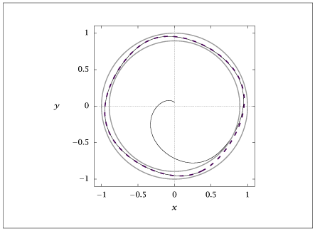
Figure 2.18:

A limit cycle (thick dashed curve) and a trajectory (thin solid curve) approaching it.

Code for Figure 2.18

Text of the GNU GPL.

main.py

 1
 2
 3
 4
 5
 6
 7
 8
 9
10
11
12
13
14
15
16
17
18
19
20
21
22
23
24
25
26
27
28
29
30
31
32
33
34
35
import numpy as np
from scipy.integrate import solve_ivp
import matplotlib.pyplot as plt

npts = 101
time = np.linspace(0, 10, npts)
z0 = np.array([0, 0.05])

def rhs(t, z):
    x = z[0]
    y = z[1]
    zdot = [x - y - x*(x**2+2*y**2), x + y - y*(x**2+y**2)]
    return zdot

sol = solve_ivp(rhs, [time[0], time[-1]], z0, t_eval=time)

z0 = sol.y[:, -1]
time = np.linspace(0, 6.5, npts)

sol_cyc = solve_ivp(rhs, [time[0], time[-1]], z0, t_eval=time)

theta = np.linspace(0, 2*np.pi, npts)
anni = np.column_stack((np.cos(theta), np.sin(theta)))
anno = 2/np.sqrt(5) * anni

traj = np.column_stack((sol.y.transpose(), sol_cyc.y.transpose(), anni, anno))

plt.figure()
plt.plot(time, sol.y.transpose())
plt.figure()
plt.plot(sol.y[0], sol.y[1], '-', sol_cyc.y[0], sol_cyc.y[1], 'o', anni[:, 0], anni[:, 1], anno[:, 0], anno[:, 1])
plt.show(block=False)

with open("cycle.dat", "w") as f:
    np.savetxt(f, traj, fmt='%f')