Figure 2.20:

A limit cycle for the R\"ossler system, a=b=0.2, c=1.

Code for Figure 2.20

Text of the GNU GPL.

main.py

 1
 2
 3
 4
 5
 6
 7
 8
 9
10
11
12
13
14
15
16
17
18
19
20
21
22
23
24
25
26
27
28
29
30
31
32
33
34
35
36
37
38
39
40
41
42
43
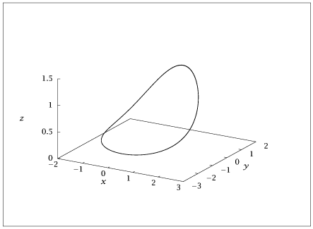
import numpy as np
from scipy.integrate import solve_ivp
import pandas as pd
import matplotlib.pyplot as plt

# Define parameters
a = 0.2; b = 0.2; c = 1
p = {'a': a, 'b': b, 'c': c}

tfin = 100
npts = 10 * tfin
time = np.linspace(0, tfin, npts)

# Define the right-hand side of the differential equation
def rhs(t, w):
    x, y, z = w
    return np.array([
        -y - z,
        x + p['a'] * y,
        p['b'] + z * (x - p['c'])
    ])

# Initial condition
w0 = [1, 1, 1]

# Solve differential equation
sol = solve_ivp(lambda t, w: rhs(t, w), [0, tfin], w0, t_eval=time, method='BDF')

# Drop the transient part
transient = round(0.8 * npts)
w = sol.y[:, transient:].T

# Save results in readable .dat format
with open("rosslercycle.dat", "w") as f:
    np.savetxt(f, w, fmt='%f', header="State Variables of Rossler Attractor")

# Plot configuration and showing plot only in interactive mode
plt.figure()
plt.plot(w)
plt.title('Rossler Attractor')
plt.xlabel('Time')
plt.ylabel('State Variables')
plt.show(block=False)