Figure 2.27:

Stability regions for Adams predictor-corrector methods; \dot {x}=\lambda x.

Code for Figure 2.27

Text of the GNU GPL.

main.py

 1
 2
 3
 4
 5
 6
 7
 8
 9
10
11
12
13
14
15
16
17
18
19
20
21
22
23
24
25
26
27
28
29
30
31
32
33
34
35
36
37
38
39
40
41
42
43
44
45
46
47
48
49
50
51
52
53
54
55
56
57
58
59
60
61
62
63
64
65
66
67
68
69
70
71
72
73
74
75
76
77
78
79
80
81
82
83
84
85
86
87
88
89
90
91
92
import numpy as np
from scipy.optimize import fsolve
import matplotlib.pyplot as plt

# Setting grid points
axisbox = [-1.5, 1.5, -1, 1]
xa, xb, ya, yb = axisbox
nhalf = 50
npts = 2*nhalf+1
theta = np.linspace(0, 4*np.pi, npts)
lamvec = np.exp(1j*theta)

# predictor coefficients, 1st, 2nd, 3rd, 4th order
p = [[1, 0, 0, 0],
     [1.5, -0.5, 0, 0],
     [23/12, -4/3, 5/12, 0],
     [55/24, -59/24, 37/24, -9/24]]

# corrector coefficients, 1st, 2nd, 3rd, 4th order
c = [[1, 0, 0, 0],
     [0.5, 0.5, 0, 0],
     [5/12, 8/12, -1/12, 0],
     [9/24, 19/24, -5/24, 1/24]]

def characteristic(w, PCs, lam):
    cc = c[PCs-1]
    pp = p[PCs-2]  # note, the predictor order is one less than corrector
    a = np.zeros(4, dtype=complex)
    a[0] = 1 + w * (cc[0] * (1 + w * pp[0]) + cc[1])
    a[1] = w * (cc[0] * w * pp[1] + cc[2])
    a[2] = w * (cc[0] * w * pp[2] + cc[3])
    a[3] = w * cc[0] * w * pp[3]
    order = len(a)
    G = np.zeros([order, order], dtype=complex)
    G[0,:] = a
    G[1:,:-1] = np.eye(order-1)
    G -= lam * np.eye(order)
    return np.linalg.det(G)

def func(w, PCs, lam):
    return [characteristic(w[0] + 1j*w[1], PCs, lam).real,
            characteristic(w[0] + 1j*w[1], PCs, lam).imag]

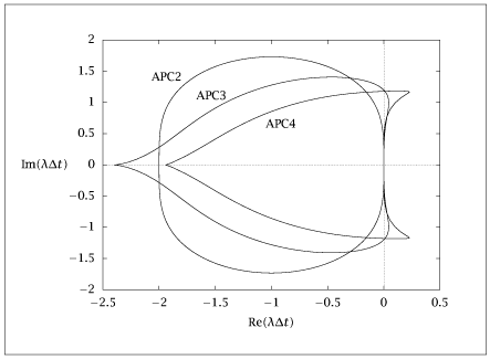
PCsvec = [2, 3, 4]
npcs = len(PCsvec)
wsol = [np.zeros(npts, dtype=complex) for _ in range(npcs)]

for j, PCs in enumerate(PCsvec):
    w0 = 0 + 0j
    for k, lam in enumerate(lamvec):
        sol = fsolve(func, [w0.real, w0.imag], args=(PCs, lam), full_output=True)
        if sol[2] == 1:
            w = sol[0][0] + 1j*sol[0][1]
            wsol[j][k] = w
            w0 = 0.95*w
        else:
            print(f"Warning: fsolve did not converge for j={j}, k={k}")
            print(sol)
wsav = wsol.copy()


# Check for intersecting loops
for ind in range(npcs):
    for k in range(len(wsol[ind]) - 1):
        z = np.array([wsol[ind].real, wsol[ind].imag])
        iloop = 0
        for j in range(k+2, len(wsol[ind])-1):
            A = np.column_stack([z[:,k]-z[:,k+1], z[:,j+1]-z[:,j]])
            if np.linalg.det(A) != 0:
                lam = np.linalg.solve(A, z[:,j+1]-z[:,k+1])
                if np.all((0 <= lam) & (lam <= 1)):
                    iloop = list(range(k+1, j+1))
                    zint = lam[0]*z[:,k] + (1-lam[0])*z[:,k+1]
                    break
        if iloop:
            zcp = complex(zint[0], zint[1])
            wsol[ind][iloop[0]] = zcp
            wsol[ind] = np.delete(wsol[ind], iloop[1:])

plt.figure()
for j in range(npcs):
    plt.plot(wsol[j].real, wsol[j].imag, '-o')
plt.show(block=False)

# Prepare data for saving

# Save to APC_stability.dat file
with open("APC_stability.dat", "w") as f:
    for j in range(npcs):
        store = np.column_stack((wsol[j].real, wsol[j].imag))
        np.savetxt(f, store, fmt='%.6f', header=f"predictor/corrector order:{j+1}/{j+2}")
        f.write("\n\n")