Figure 2.4:

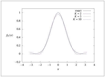
Function f(x)=\exp \big (-8\big (\frac {x}{\pi }\big )^{2}\big ) and truncated trigonometric Fourier series approximations with K=2,5,10. The approximations with K=5 and K=10 are visually indistinguishable from the exact function.

Code for Figure 2.4

Text of the GNU GPL.

main.m

 1
 2
 3
 4
 5
 6
 7
 8
 9
10
11
12
13
14
15
16
17
18
19
20
21
22
23
24
25
26
27
28
29
30
31
32
33
34
35
36
37
38
% Fourier series of a Gaussian function
% (after JBR solution)
%MDG 12/3/12

nxs = 1000; % number of points
x = linspace(-pi, pi, nxs); %points for plotting
dx=2*pi/(nxs-1); %spacing between points
nterms = [2,5,10]; % number of terms for sums
u = zeros(length(nterms), nxs);
ntermsmax=nterms(length(nterms));
phi=zeros(ntermsmax,nxs);
%generate basis functions
phi(1,:)=1/sqrt(2*pi);
for m=1:ntermsmax
    phi(m+1,:)=1/sqrt(pi)*cos(m*x);
end
% n=1;
% plot(x,phi(n+1,:)) % plot nth basis fn (recalling that indices start at
% % 0
% generate function at points x
flist=exp(-8/pi^2*x.^2);
% plot(x,flist)
for i = 1:length(nterms)
  for k = 0:nterms(i);
      % compute coefficients by simple rectangle rule sum
      % (quick and dirty, but inaccurate for large k, because of the
      % oscillations of the basis functions)

        ck = dot(flist(:),phi(k+1,:))*dx;
        u(i,:) = u(i,:)+ ck*phi(k+1,:);
  end
end
plot(x,flist,'-',x,u(1,:),'--',x,u(2,:),':',x,u(3,:),'-.');
legend('exp(-8x^2/pi^2)','K=2','K=5','K=10');

%save results for plotting with gnuplot
table = [x' flist' u'];
save FourierGaussian.dat table