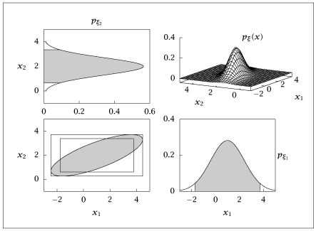
importnumpyasnpfromnumpy.linalgimportinvfromscipy.statsimportchi2fromscipy.linalgimportsqrtmimportmatplotlib.pyplotaspltfrommiscimportellipse# Set parametersm=np.array([[1],[2]])n=len(m)P=np.array([[2,0.75],[0.75,0.5]])nsam=1000np.random.seed(0)# Generate samplesx=np.tile(m,(1,nsam))+sqrtm(P)@np.random.randn(n,nsam)# Compute the 95% confidence interval ellipsealpha=0.95A=inv(P)b=chi2.ppf(alpha,n)xe,ye,*_=ellipse(A,b,100,m)# Count how many samples are outside the ellipsee=x-np.tile(m,(1,nsam))outside_ellipse=np.sum(np.diag((e.T@A)@e)>b)/nsam# Compute the 95% bounding boxxd=np.sqrt(b*np.diag(P))bbox=np.array([[-xd[0],-xd[1]],[xd[0],-xd[1]],[xd[0],xd[1]],[-xd[0],xd[1]],[-xd[0],-xd[1]]])bbox=bbox+np.tile(m.T,(5,1))# Count samples outside the bounding boxz=x-np.tile(m,(1,nsam))outside_bbox=sum(sum(np.abs(z)>xd[:,None])>0)/nsam# Compute 95% marginal intervalsb2=chi2.ppf(alpha,1)xd2=np.sqrt(b2*np.diag(P))mbox=np.array([[-xd2[0],-xd2[1]],[xd2[0],-xd2[1]],[xd2[0],xd2[1]],[-xd2[0],xd2[1]],[-xd2[0],-xd2[1]]])mbox=mbox+np.tile(m.T,(5,1))# Count samples outside the marginal boxoutside_mbox=sum(sum(np.abs(z)>xd2[:,None])>0)/nsam# Prepare mtab data (xplot, fx for both components)xrange=np.round([np.min(x,axis=1),np.max(x,axis=1)]).astype(int).Tnplot=100xplot=np.linspace(xrange[:,0],xrange[:,1],nplot).Tz=xplot-mdiagP=np.diag(P)[:,None];fx=np.exp(-(1/2)*(z/diagP*z))/np.sqrt(2*np.pi*diagP)# compute closed curves for using filledcurve in gnuplotind=abs(z)<=xd2[:,None]xp1=xplot[0,:]xp2=xplot[1,:]fx1=fx[0,:]fx2=fx[1,:]ind1=ind[0,:]ind2=ind[1,:]fill1=np.row_stack((xp1[ind1],fx1[ind1]))fill1=np.column_stack((np.row_stack((fill1[0,0],0)),fill1,np.row_stack((fill1[0,-1],0)))).Tfill2=np.row_stack((xp2[ind2],fx2[ind2]))fill2=np.column_stack((np.row_stack((fill2[0,0],0)),fill2,np.row_stack((fill2[0,-1],0)))).Tnbins=20# Histogram for x[0,:]n1,bins1=np.histogram(x[0,:],bins=nbins,density=True)bin_centers1=0.5*(bins1[:-1]+bins1[1:])# make bar plot data for gnuplotbarx1=np.kron(bins1,[1,1,1])[1:-1]bary1=np.append(np.kron(n1,[0,1,1]),0)# Histogram for x[1,:]n2,bins2=np.histogram(x[1,:],bins=nbins,density=True)bin_centers2=0.5*(bins2[:-1]+bins2[1:])# make bar plot data for gnuplotbarx2=np.kron(bins2,[1,1,1])[1:-1]bary2=np.append(np.kron(n2,[0,1,1]),0)plt.figure()plt.plot(x[0,:],x[1,:],'o',mfc='none')plt.plot(xe,ye)plt.plot(bbox[:,0],bbox[:,1])plt.plot(mbox[:,0],mbox[:,1])plt.figure()plt.plot(barx1,bary1,label='Histogram x[1,:]')plt.figure()plt.plot(barx2,bary2,label='Histogram x[2,:]')plt.figure()plt.plot(xplot[0,:],fx[0,:])plt.plot(xplot[1,:],fx[1,:])plt.show(block=False)samtab=x.Teltab=np.column_stack([xe,ye])mtab=np.column_stack((xplot.T,fx.T))# Create the .dat file with correct formatting for Gnuplotwithopen("confmarg.dat","w")asf:# Write sample matrix (samtab)np.savetxt(f,samtab,fmt='%f',header="samtab")f.write("\n\n")# Write ellipse data (eltab)np.savetxt(f,eltab,fmt='%f',header="eltab")f.write("\n\n")# Write ellipse data (eltab)np.savetxt(f,mtab,fmt='%f',header="mtab")f.write("\n\n")# Write bounding box data (bbox)np.savetxt(f,bbox,fmt='%f',header="bbox")f.write("\n\n")# Write marginal box data (mbox)np.savetxt(f,mbox,fmt='%f',header="mbox")f.write("\n\n")# Write fill1 and fill2 datanp.savetxt(f,fill1,fmt='%f',header="fill1")f.write("\n\n")np.savetxt(f,fill2,fmt='%f',header="fill2")