Figure 4.18:

Smooth approximation to a unit step function, H(z-1).

Code for Figure 4.18

Text of the GNU GPL.

main.py

 1
 2
 3
 4
 5
 6
 7
 8
 9
10
11
12
13
14
15
16
17
18
19
20
21
22
23
24
25
26
27
28
29
30
31
32
33
34
35
36
37
38
39
40
41
42
43
44
45
46
47
48
49
50
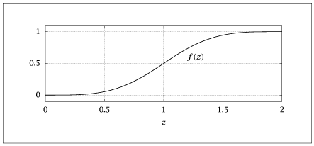
import numpy as np
import matplotlib.pyplot as plt

# Set parameters
L = 2
r = L / 2

# Number of points and x values
npts = 51
x = np.linspace(0, L, npts)

# Function definitions
f1 = (1/4)*(5*(x/r)**4 - 3*(x/r)**5)
z = (2*r - x)/r
f2 = -(1/4)*(5*z**4 - 3*z**5) + 1
f = np.where(x <= r, f1, f2)

# First derivative
df1 = (1/(4*r))*(20*(x/r)**3 - 15*(x/r)**4)
df2 = (1/(4*r))*(20*z**3 - 15*z**4)
df = np.where(x <= r, df1, df2)

# Second derivative
d2f1 = (1/(4*r**2))*(60*(x/r)**2 - 60*(x/r)**3)
d2f2 = -(1/(4*r**2))*(60*z**2 - 60*z**3)
d2f = np.where(x <= r, d2f1, d2f2)

# Third derivative
d3f1 = (1/(4*r**3))*(120*(x/r) - 180*(x/r)**2)
d3f2 = (1/(4*r**3))*(120*z - 180*z**2)
d3f = np.where(x <= r, d3f1, d3f2)

# Plotting
plt.figure()
plt.plot(x, f, '-o')
plt.title('Function f')
plt.figure()
plt.plot(x, df, '-o')
plt.title('First Derivative df')
plt.figure()
plt.plot(x, d2f, '-o')
plt.title('Second Derivative d2f')
plt.figure()
plt.plot(x, d3f, '-o')
plt.title('Third Derivative d3f')
plt.show(block=False)

# Save data to file
smooth = np.column_stack((x, f, df, d2f, d3f))
np.savetxt('indscaled.dat', smooth, fmt='%f')