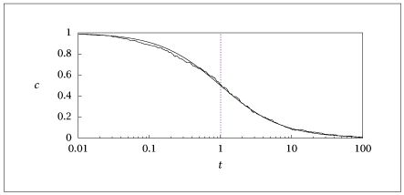
Figure 5.14:

Simulation of 2 A \mathrel {\mkern 4mu}\mathrel {\smash {\mathchar "392D}}\mathrel {\mkern -2.5mu}-> B for n_0=500, \Omega =500. Top: discrete simulation; bottom: SDE simulation.

Code for Figure 5.14

Text of the GNU GPL.

main.py

 1
 2
 3
 4
 5
 6
 7
 8
 9
10
11
12
13
14
15
16
17
18
19
20
21
22
23
24
25
26
27
28
29
30
31
32
33
34
35
36
37
38
39
40
41
42
43
44
45
46
47
48
49
50
51
52
53
54
55
56
57
58
59
60
61
62
import numpy as np
import matplotlib.pyplot as plt

omega = 500
k = 1
c0 = 1
n0 = int(c0 * omega)

nsim = 10 * omega
time = np.zeros(nsim + 1)
time[0] = 0
n = np.zeros(nsim + 1)
n[0] = n0
np.random.seed(10)
for i in range(nsim):
    r = k * n[i] * (n[i] - 1) / (2 * omega)
    if r == 0:
        n = n[:i + 1]
        time = time[:i + 1]
        break
    tau = -np.log(np.random.rand()) / r
    time[i + 1] = time[i] + tau
    n[i + 1] = n[i] - 2

nts = 500
tinit = 1e-2
tfin = 1e2
tc = np.logspace(np.log10(tinit), np.log10(tfin), nts)
c = 1 / (1 / c0 + k * tc)

xi = np.zeros(nts)
np.random.seed(0)
for i in range(nts - 1):
    Delta = tc[i + 1] - tc[i]
    xi[i + 1] = xi[i] - 2 * k * c[i] * xi[i] * Delta + np.sqrt(2 * k * c[i] * c[i] * Delta) * np.random.randn()
csde = c + xi / np.sqrt(omega)

plt.figure()
ts, ns = time, n
cs = ns / omega
plt.semilogx(ts, cs, label='kMC Simulation', base=10)
plt.semilogx(tc, c, label='Deterministic Solution', base=10)
plt.axis([tinit, tfin, 0, 1])
plt.legend()
plt.show(block=False)

plt.figure()
plt.semilogx(tc, csde, label='SDE Approximation', base=10)
plt.semilogx(tc, c, label='Deterministic Solution', base=10)
plt.axis([tinit, tfin, 0, 1])
plt.legend()
plt.show(block=False)

ts_ns_length = len(ts) - 1
tc_twice = np.tile(tc, 2)
c_twice = np.tile(c, 2)
csde_twice = np.tile(csde, 2)

data = np.column_stack((ts[:-1], cs[:-1], tc_twice[:ts_ns_length], c_twice[:ts_ns_length], csde_twice[:ts_ns_length]))

with open("sam2nd.dat", "w") as f:
    np.savetxt(f, data, fmt='%f')