Figure 5.15:

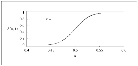
Cumulative distribution for 2 A \mathrel {\mkern 4mu}\mathrel {\smash {\mathchar "392D}}\mathrel {\mkern -2.5mu}-> B at t=1 with n_0=500, \Omega =500. Discrete master equation (steps) versus omega expansion (smooth).

Code for Figure 5.15

Text of the GNU GPL.

main.py

 1
 2
 3
 4
 5
 6
 7
 8
 9
10
11
12
13
14
15
16
17
18
19
20
21
22
23
24
25
26
27
28
29
30
31
32
33
34
35
36
37
38
39
40
41
42
43
44
45
46
47
48
49
50
51
52
53
54
55
56
57
58
59
60
61
62
63
64
65
66
67
68
69
70
71
72
73
74
75
76
77
78
79
80
81
82
83
84
85
86
87
88
89
90
91
92
93
94
95
import numpy as np
from scipy.linalg import expm, solve_banded
from scipy.special import erfc
from scipy.sparse import diags
import matplotlib.pyplot as plt
from misc import colloc
from scikits.odes import dae

# Parameters
omega = 500
k = 1
c0 = 1
n0 = int(c0 * omega)
b = 3

ncol = 25;
x, A, B, q = colloc(ncol-1, left=True)
x = b*x;
A = A/b;
B = B/(b*b);
q = q*b;

def continuous(t, F, Fdot, resid):
    """Residual function for the DAE system."""
    c = 1 / ( 1/c0 + k*t )
    v = -2 * k * c * x
    D = k * c * c
    Fx = A @ F
    dFdt = -v * Fx + D * B @ F
    resid[0:] = Fdot - dFdt
#    resid = Fdot - dFdt
    resid[0] = F[0] - 0.5
    resid[-1] = F[-1] - 1

# Time parameters
tstop = 1
nts = 25
tsteps = np.linspace(0, tstop, nts)
var = 1e-2

# Initial conditions
y0 = 0.5 * erfc(-x / (np.sqrt(2) * 5 * var))
ydot0 = np.zeros(ncol)
resid = np.zeros(ncol)
continuous(0, y0, ydot0, resid)
ydot0 = -resid
ydot0[0] = 0

solver = dae('ida', continuous,
             compute_initcond='yp0',
             first_step_size=1e-6,
             atol=1e-6,
             rtol=1e-6,
             algebraic_vars_idx=[0,-1],
             old_api=False)

solution = solver.solve(tsteps, y0, ydot0)
y = solution.values.y

# Final adjustments
cstop = 1 / (1 / c0 + k * tstop)
xshift = np.concatenate([-np.flipud(x), x]) / np.sqrt(omega) + cstop
F = np.concatenate([1 - np.flipud(y[-1, :]), y[-1, :]])

# Stochastic simulation
n = np.arange(n0 + 1)
d1 = -k * n * (n - 1) / (2 * omega)
d2 = k * (n + 2) * (n + 1) / (2 * omega)
A = diags([d1, d2[:-2]], [0, 2]).toarray()
P0 = np.zeros_like(n)
P0[-1] = 1
P = expm(A * tstop) @ P0
Fmas = np.cumsum(P)

nscal = n / omega

# Plotting
plt.figure()
plt.plot(nscal, Fmas, label='Master Equation')
plt.plot(xshift, F, label='PDE')
plt.axis([0.4, 0.6, 0, 1])
plt.legend()

plt.figure()
plt.plot(nscal, Fmas, label='Master Equation')
plt.plot(xshift, F, label='PDE')
plt.legend()

plt.show(block=False)

# Save results
with open("F2nd.dat", "w") as f:
    np.savetxt(f, np.vstack((nscal, Fmas)).T, fmt='%f', header="Master Equation")
    f.write("\n\n")
    np.savetxt(f, np.vstack((xshift, F)).T, fmt='%f', header="PDE")