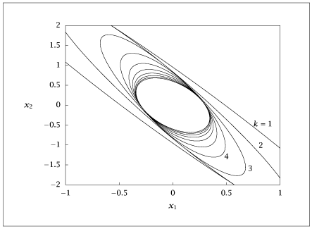
← Back to Figures Figure 5.16:
The change in 95% confidence intervals for \hat {x}(k\vert k) versus time for a stable, optimal estimator. We start at k=0 with a large initial variance P(0), which gives a large confidence interval.
Code for Figure 5.16
Text of the GNU GPL .
main.py
1
2
3
4
5
6
7
8
9
10
11
12
13
14
15
16
17
18
19
20
21
22
23
24
25
26
27
28
29
30
31
32
33
34
35
36
37
38
39
40
41
42
43
44
45
46
47
48
49
50
51
52
53
54
55
56
57
58
59
60
61 # [depends] ~/pythonlib/misc.py
import numpy as np
import matplotlib.pyplot as plt
from scipy.stats import chi2
from scipy.linalg import inv
from misc import ellipse
ntsteps = 10
U = 0.5 * np . array ([[ np . sqrt ( 2 ), np . sqrt ( 2 )], [ np . sqrt ( 2 ), - np . sqrt ( 2 )]])
theta = ( - 25 ) * 360 / ( 2 * np . pi )
A = np . array ([[ np . cos ( theta ), np . sin ( theta )], [ - np . sin ( theta ), np . cos ( theta )]])
n = A . shape [ 0 ]
C = np . array ([[ 0.5 , 0.25 ]])
G = np . eye ( 2 )
m = 2
B = np . eye ( m )
g = G . shape [ 1 ]
p = C . shape [ 0 ]
alpha = 0.95
nell = 281
bn = chi2 . ppf ( alpha , n )
prior = 3
Q0 = prior * np . eye ( n )
Q = 0.01 * np . eye ( g )
R = 0.01 * np . eye ( p )
Pminus = [ Q0 ]
L = np . zeros (( ntsteps , 2 , 1 ))
P = np . zeros (( ntsteps , 2 , 2 ))
exm = np . zeros (( ntsteps , nell , 2 ))
ex = np . zeros (( ntsteps , nell , 2 ))
for i in range ( ntsteps ):
C_Pminus_Ct = C @ Pminus [ i ] @ C . T
L [ i ] = Pminus [ i ] @ C . T @ inv ( R + C_Pminus_Ct )
P [ i ] = Pminus [ i ] - L [ i ] @ C @ Pminus [ i ]
exm [ i ][:, 0 ], exm [ i ][:, 1 ], * _ = ellipse ( inv ( Pminus [ i ]), bn , nell )
ex [ i ][:, 0 ], ex [ i ][:, 1 ], * _ = ellipse ( inv ( P [ i ]), bn , nell )
if i == ntsteps - 1 :
break
Pminus . append ( A @ P [ i ] @ A . T + G @ Q @ G . T )
plt . figure ()
for i in range ( ntsteps ):
plt . plot ( ex [ i ][:, 0 ], ex [ i ][:, 1 ])
plt . axis ([ - 1 , 1 , - 2 , 2 ])
plt . show ( block = False )
plt . figure ()
for i in range ( ntsteps ):
plt . plot ( exm [ i ][:, 0 ], exm [ i ][:, 1 ])
plt . show ( block = False )
with open ( "KFpayoff.dat" , "w" ) as f :
for i in range ( ntsteps ):
np . savetxt ( f , ex [ i ], fmt = ' %f ' )
f . write ( " \n\n " )