Figure 5.4:

The mean square displacement versus time; D=2, V=0, n=500.

Code for Figure 5.4

Text of the GNU GPL.

main.py

 1
 2
 3
 4
 5
 6
 7
 8
 9
10
11
12
13
14
15
16
17
18
19
20
21
22
23
24
25
26
27
28
29
30
31
32
33
34
35
36
37
38
39
40
41
42
43
44
45
46
47
48
49
50
51
52
53
54
55
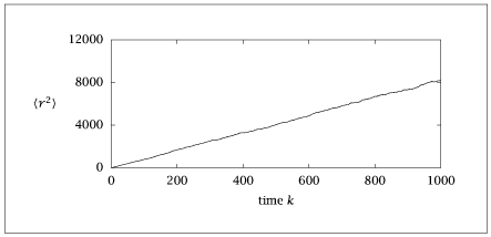
import numpy as np
import matplotlib.pyplot as plt

tfinal = 1000
time = np.arange(tfinal + 1)
ntimes = len(time)
npart = 500
ndim = 2
D = 2
v = 0  # drift term is v_x=v, v_y=v

np.random.seed(0)

x = np.zeros((ntimes, npart, ndim))
S = np.zeros((ntimes, npart, ndim))
rsq = np.zeros((ntimes, npart))
drsqD = np.zeros((ntimes, npart))

for i in range(ntimes-1):
    ranstep = np.sqrt(2*D)*np.random.randn(npart, ndim)
    location = x[i, :, :] + v + ranstep
    x[i+1, :, :] = location
    partial = S[i, :, :] + 1/(2*D)*ranstep
    S[i+1, :, :] = partial
    rsq[i+1, :] = np.sum(location**2, axis=1)
    drsqD[i+1, :] = 2 * np.sum(location * partial, axis=1)

mrsq = np.mean(rsq, axis=1)
dmrsqD = np.mean(drsqD, axis=1)

# Plot the mean of the r^2 displacement
plt.figure()
plt.plot(time, mrsq)
plt.show(block=False)

# Plot the derivative with respect to diffusivity of the mean of the r^2 displacement
plt.figure()
plt.plot(time, dmrsqD)
plt.show(block=False)

# Plot a typical particle trajectory
plt.figure()
particle = 1
traj = x[:, particle, :]
plt.plot(traj[:, 0], traj[:, 1], '-o', mfc='none')
plt.show(block=False)

# Save data into a single .dat file

data1 = np.column_stack((time, mrsq, dmrsqD))

with open("brownian2d.dat", "w") as f:
    np.savetxt(f, data1, fmt='%f', header="data1")
    f.write("\n\n")
    np.savetxt(f, traj, fmt='%f', header="trajectory")