Shear Flow Simulation: Velocity Field, Flow Boundary Conditions and Flow Structure
Chia-Chun Fu
CHE210D Spring 2009 Final Project
Summary
Molecular dynamics simulations are carried out to investigate Lennard-Jones liquids sheared between two solid walls. Velocity profiles, flow boundary conditions and flow structures were studied for various wall-fluid interactions. For weak wall-fluid interactions, the flow structure is less ordered and slip was observed. For larger wall-fluid interactions, the flow structure is more ordered and the first one or two fluid layers near the walls were moving with the wall.
Background
In order to describe the fluid flow in confined geometry, it requires “no-slip” boundary condition for the fluid velocity at the solid wall. The assumption successfully describes fluid flow on macroscopic length scales; however, it has to be revised for microscopic length scales due to the possible slip between fluid and wall. By performing MD simulation, the fluid velocity profile can be resolved at molecular level and no assumption at interface is required.
Simulation methods
The simulations were performed in a Couette geometry with two walls parallel to xy plane. Each wall consisting two planes of fcc lattice moved with constant velocity Uupper=-1, -2 and Ulower=1, 2. The interactions between fluid atoms were using a Lennard-Jones potential,
VLJ(r) = 4 ε [(σ/r)12 — (σ/r)6],
where r is distance between atoms, and ε and σ are characteristic energy and length scales of the fluid. For LJ interactions between fluid and wall atoms, energy and length scale εwf (=ε, 0.4ε, and 4ε) and σwf (=σ) were used. The temperature and density of the fluid were fixed at kBT/ε = 1.1 and ρσ3 = 0.81. Also, ρwall = ρ. Other settings state below:
· Nupper = 96
· Nlower = 96
· Nfluid = 720
· rc = 2.2σ
· bin size » 0.7298 σ
· Lattice space = (4/ρ)1/3
· Dt = 0.005
· 60,000 integration steps (t=0 to t=300, collect data after t=250)
When ρσ3 = 0.81, the system measures h = 13.62σ between the walls, and 13.62 σ by 5.11σ in the xy plane. Velocity Verlet algorithm and velocity rescaling were used with periodic boundary conditions imposed along x and y axes. The initial velocities of fluid atoms were generated from a normal distribution with m=0 and s=(3.3)0.5 3.
 .
.
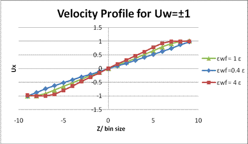
Figure 1. Velocity profile for ρσ3 = 0.81, Uw = ±1 and bin size=0.7298σ. For εwf= 4 ε, we can see the first two layers near the wall have the same velocity as the wall. And for εwf= 0.4 ε, the velocity profile is linear with a no-slip boundary condition.
 .
.
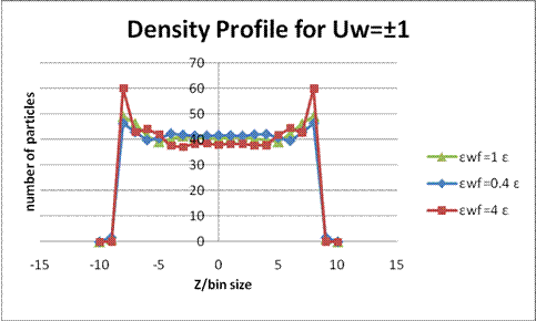
Figure 2. Density profile for ρσ3 = 0.81, Uw = ±1 and bin size=0.7298σ. For εwf= 4 ε, atoms tend to form layers near the wall.
 .
.
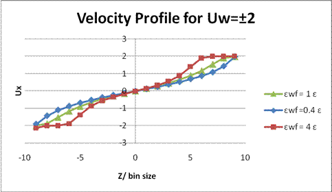
Figure 3. Velocity profile for ρσ3 = 0.81, Uw = ±2 and bin size=0.7298σ. While Uw become ±2, no-slip boundary condition is not valid for these three ratio of wall-fluid interactions.
 .
.
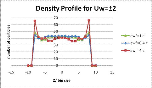
Figure 4. Density profile for ρσ3 = 0.81, Uw = ±2 and bin size=0.7298σ. Compare to the case of Uw = ±1 [Fig. 2.], the fluid structures are similar except for the enhanced density oscillation of εwf= 4 ε.
 .
.
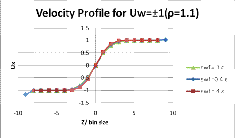
Figure 5. Velocity profile for ρσ3 = 1.1, Uw = ±1 and bin size=0.7298σ. For high density, the fluid is acting more like a solid. For higher wall-fluid interaction, no fluid atoms can go into the first bin because of the higher repulsion near the wall (< 1.12 σ).
 .
.
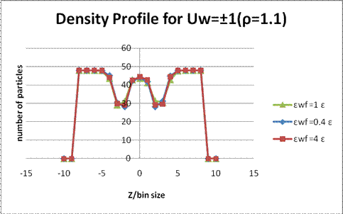
Figure 6. Density profile for ρσ3 = 1.1, Uw = ±1 and bin size=0.7298σ. The density profiles near the wall are not as sharp as the case of lower density. Also, because it is more solid-like, atoms are moving together and the fluid layers become wider.
 .
.
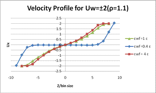
Figure 7. Velocity profile for ρσ3 = 1.1, Uw = ±2 and bin size=0.7298σ.Compare to Uw = ±1, the velocity profiles are very different, but still no atom can go into the first bin near the wall for higher wall-fluid interaction.
 .
.
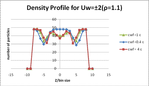
Figure 8. Density profile for ρσ3 = 1.1, Uw = ±2 and bin size=0.7298σ. Compare to Uw = ±1, the fluid structures are similar but the density oscillations are enhanced. The same tendency also occurs in ρσ3=0.81.
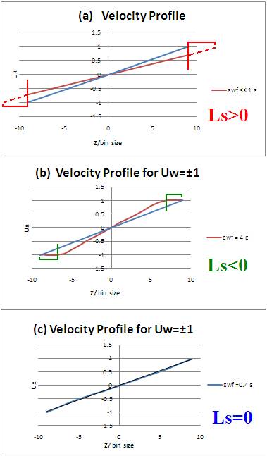
Figure 9. In the reference, a length Ls was defined to characterize the degree of slip. When εwf<< 1 ε, the slip boundary will occur and Ls will be positive (a). The usual no-slip boundary corresponds to Ls=0 (c). And for Ls<0 (b), there are fluid layers moving with the wall.
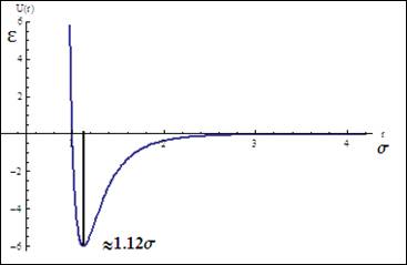
Figure 10. Potential energy vs. the distance between atoms. The value labeled shows the distance where the force (derivative of potential energy) between two atoms is zero.
Results and interpretation
a. Velocity profiles
The simulations ran for two different wall velocities, three kinds of wall-fluid interaction energies and two different densities. First, a length Ls was defined to evaluate the results [Fig. 9.]. For Uw=±1[Fig. 1.], only εwf= 0.4 ε showed the no-slip boundary condition is valid and the stronger wall- fluid interactions gave negative values of Ls, which means there were fluid layers formed near the walls. For Uw= ±2 [Fig. 3.], the middle parts of curves were not linear, which could be caused by rising the wall velocity but still keeping the same time step. Fluid in the middle cannot immediately respond to the velocity change at the boundary before the next move. Also, while the higher wall velocity gave more fluctuations, the production period might not be long enough to show better averages. For fixed temperature and density, kBT/ε = 1.1 and ρσ3 = 0.81, the fluid is about 30% above the melting temperature. Therefore, when ρσ3 = 1.1, the compressed fluid behaved more like a solid, which was shown in Fig. 5 and Fig 7. The major difference between these two figures might be due to the same reason that the wall was moving faster with same time step and the momentum did not perfectly transfer to the middle part of fluid for the case of εwf= 0.4 ε. One of the interesting results shown in these two figures is that no fluid atom can go into the first bins near the walls when the wall-fluid interaction was stronger. As we know, higher wall-fluid coupling will give higher repulsion and attraction between wall and fluid. From Fig. 10, we can find the distance where the force between two atoms is zero, r»1.12s. Also, we know that the bin size is around 0.73s. Therefore, due to the large repulsive force, the wall and fluid atoms cannot approach to each other in the first bins.
b. Density profiles
The oscillations of density profile are induced by the structure of the fluid pair correlation function g(r) and the wall potential. The wall potential gives the sharp cutoff of fluid density at the boundary. From Fig. 2 and Fig. 4, the sharp fluid layers at the walls only occurred when the wall-fluid coupling is stronger, such as εwf= 4 ε. Also, the competition between two length scales, wall- fluid and fluid-fluid, affects the amplitude of the oscillations. While the density became higher, the fluid layers became wider [Fig. 6 and 8]. The lower the wall velocity was, the wider the fluid layers were [Fig. 2, 4, 6 and 8].
c. Deficiencies of the model
While velocity rescaling does not capture the correct energy fluctuations, other advanced thermostats, such as Langevin or Andersen thermostat, should be applied to give better dynamics and statistical properties. Also, my model is simplified by neglecting the thermal roughness of the wall and just making the walls moving with constant velocities. It will be more close to the real model if the spring constant was added back to the wall atoms.
Movies
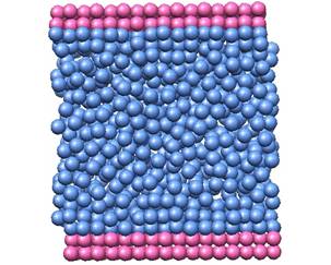
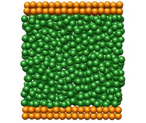
Figure 11. Movie for ρσ3 = 0.81, Uw = ±1, εwf= 4 ε Figure 12. Movie for ρσ3 = 0.81, Uw = ±1, εwf=0.4 ε
From the two movie snaps, it is obvious that the first two layers of fluid are moving with the wall and more atoms accumulate at the boundary for strong wall-fluid coupling [Fig.11.] and no ordered layer is formed near the wall and atoms tend to be less ordered for weaker wall-fluid interaction [Fig. 12.]. Both of the movies consist with the results stated at the former section.
Source code
References
Peter A. Thompson and Mark O. Robbins, Phys. Rev. A, Volume 41, Number 12 (1990)
“Shear Flow near solids: Epitaxial order and flow boundary conditions”
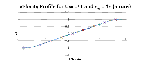
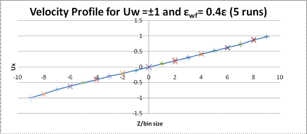
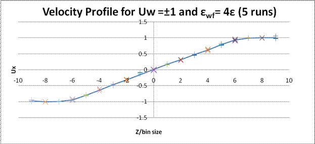
More graphs
These are graphs of velocity profile for multiple simulations with different wall-fluid interactions.
I have tried to add error bars (from standard deviation) on these graphs; however, they were too small to show on the graphs. Therefore, I didn’t put these graphs at the former part but attached them here. Standard deviation of velocity in each bin was shown in Excel file.
 .
.
 .
.
 .
.