Radius of gyration of a polymer
Edmund Lin
CHE210D Spring 2009 Final Project
Summary
The radius of gyration is easy to compute, and is often invoked in studying small dynamic systems. For example, the radius of gyration measures the effective size of a polymer. As we’ve seen in an earlier exercise, the radius of gyration can be used to quantify the degree of folding in proteins due to the hydrophobic effect.
Background
The radius of gyration is often used to characterize the dynamic trajectory of flexible systems for molecular systems. Here, a small radius of gyration indicates the polymer is relatively compact, meaning throughout its trajectory the polymer spends most of its time as a folded structure. We can measure the distribution of the radius of gyration of a polymer’s dynamic trajectory to characterize folding patterns.
Simulation methods
For this simulation exercise, I ran a canonical MD simulation of a linear Lennard-Jones polymer with a reasonable length of 20 atoms. Each atom in polymer interact with each other through L-J and harmonic spring potential. Each simulation ran for 100,000 MD time steps with the Verlet integrating scheme, and allowed to equilibrate. The radius of gyration for the polymer is monitored at different temperatures, and is averaged over 10 production runs. Simulations are carried out for T = 1.0, 2.5, 5.0, 7.5, and 10.0. The radius of gyration is expected to be between 0 and 10. A histogram of 100 bins is constructed based on these limits.
Results and interpretation
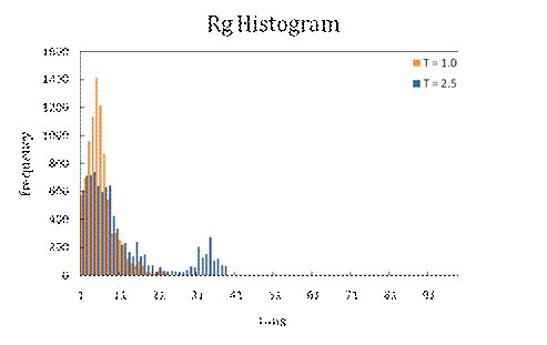
The results are plotted for different dimensionless temperatures.

Figure 1. Rg Histogram for a 20-atom L-J polymer at T = 1.0 and T = 2.5.
When I increase the temperature, the polymers tend to have higher radius of gyration. For the lowest temperatures, the higher one has two predominant frequencies. Two maxima in the distribution indicates a two-stated polymer collapse where the polymer has two predominant conformations.1 The histogram for the radius of gyration at higher temperatures is shown below.

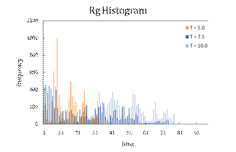
Figure 2. Rg Histogram for 20-atom L-J polymer at T = 5.0, T = 7.5, and T = 10.0.
From Figure 2, the average radius of gyration is higher for polymers at higher temperatures. This indicates polymers tend to be relatively unfolded. Also, another important point to notice is that the maximum peaks tend to shift from lower to higher radius of gyration in the following way: there is one prominent distribution of peaks at extreme temperatures, whereas at intermediate temperatures the distribution is spread over two distinct peaks. This indicates there is an intermediate ‘folding temperature’ where a polymer folds from a folded state to an unfolded state. These polymers are termed ‘two-state’ folders.
The margin of error for each simulation is large, some on the same order of magnitude as the frequency itself. My best guess is that the errors are associated with the distribution function itself since the radius of gyration is measured at every time-step. We can better the simulation averages by computing the radius of gyration at a given frequency of steps, and running longer production runs. Another possible issue with the histogram is the choice of bin width, the appropriate bracket of the maximum and minimum radius of gyration, and polymer length. We can tune these parameters to filter out the amount of fluctuations in the radius of gyration.
Generally, the correlation between structure and the radius of gyration is incorrect, but it provides a quantitative way to measure the distribution of structures as it folds.
Movies
Source code