Phase Separation in Block Copolymer Melts

Zoltan Mester

CHE210D Spring 2009 Final Project

Summary

Molecular dynamics simulations are carried out on polymer chains made up of all A or B monomers with hydrogen bonding head groups, and phase segregation is characterized via radial distribution functions. The radial distribution functions confirm that phase segregation is stronger at lower temperatures, with nearly complete phase segregation at T=1.2. At high temperature (T=2), the radial distribution functions are qualitatively similar to that of a mix of Lennard-Jones particles in the liquid phase that do not phase separate, suggesting low segregation.

Background

Supramolecular copolymers use non-covalent bonds, such as hydrogen bonds, to reversibly tether functional polymeric units into large macromolecules [1]. This is useful because material properties that depend on the connectivity of the polymers, such as phase behavior, can be studied with this model [1]. I propose a model of chains made up of all A and B monomers with favorable interactions between like monomers and head groups that interact via hydrogen bonds regardless of the identity of the chains to look for evidence of chain segregation at a few sample temperatures.

Simulation methods

Two different types of polymers consisting of A and B type monomers with reversibly hydrogen bonding head groups, H, in the melt phase are studied. The hydrogen bonding is modeled via a 10-12 Lennard-Jones potential with e_HH=20*e, and the directionality of hydrogen bonding is ignored. The polymer chains consist of 7 A or B beads plus 1 hydrogen bonding bead with e_AH’=e_BH’=e_AB=0.2*e and e_AH=e_BH=e_AA=e_BB=e, and a 6-12 Lennard-Jones potential is used for all the non-HH interactions. Here, the apostrophe indicates a hydrogen group on a chain of the opposite type. The interactions between adjacent beads on the same polymer are harmonic with a spring constant k=3000 and equilibrium length r₀=1. There are an equal number of A and B chains in the system.

 

The simulation is molecular dynamics with the velocity Verlet algorithm. The NVT ensemble is enforced via the Anderson thermostat using massive collisions.

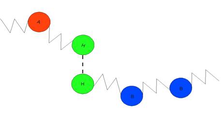
Figure 1: Bead-Spring Model

Results and interpretation

The A-A and H-H radial distribution functions of the melt at high temperature (T=2) qualitatively follow the A-A radial distribution function of a 6-12 Lennard-Jones liquid mixture with no phase separation (i.e. all monomer interactions are the same) indicating an essentially disordered system (Figure 2). The intermediate temperature (T=1.5) radial distribution functions show some qualitative differences with that of the liquid indicating some phase segregation (Figure 3). The radial distribution functions for T=1.2 (Figure 4) show strong differences between that of the disordered liquid indicating a highly segregated regime, which is confirmed by the movie. While all the distribution functions have a higher maximum peak than the liquid, partly due to the chain conformations, at low temperatures these peaks are much higher, indicating close proximity of like monomers without unlike monomers between them.  The other qualitative differences between the radial distribution functions of the low temperature melt and the high temperature melt also indicate a different underlying order from complete mixing.

 

At low temperatures, the energetic interactions between beads dominate, which favor phase segregation. In addition, the hydrogen bonds become nearly irreversible due to their bonding energy being significantly higher than the beads’ kinetic energy. As temperature becomes higher, the kinetic energy can overcome the interactions between beads causing a more disordered state. The hydrogen bonds also become reversible with higher temperature. Thus, at low temperature the system’s energetic interactions dominate while at higher temperature the equilibrium structure is more due to entropic effects.  

 

The model can be improved by adding directionality to the hydrogen bonds. In addition, the hydrogen bonding interactions can be restricted to only the head groups of chains made up of different monomers to offer a better comparison to previously done theoretical studies [1,2].

Movie

block_copolymers_zoltan_mester_small_radius.avi

The movie consists of a clip showing the evidence of phase segregation at a dimensionless temperature of 1.2. The hydrogen bonding head groups are the green beads and the A and B beads are red and blue, respectively. The head groups aggregate due to the strong hydrogen bonding interactions and the A and B chains segregate due to the more favorable interaction of like monomers.

Source code

source.zip

References

[1] W.B. Lee, R. Elliott, K. Katsov, and G.H. Fredrickson, Macromol. 40, 8445 (2007).

[2] E.H. Fang, W.B. Lee, G.H. Fredrickson, Macromol. 40, 693 (2007).

Figures

 

Figure 2: A-A and H-H radial distribution functions for the polymer melt at T=2 and the A-A distribution function for the disordered liquid mixture. The liquid mixture has the same proportion of A, B, and H particles as the polymer melt. The radial distribution functions not included are ones that have the same quantitative behavior as the ones already present.

 

 

Figure 3: A-A and H-H radial distribution functions for the polymer melt at T=1.5 and the A-A distribution function for the disordered liquid mixture at T=2.

 

 

Figure 3: A-A and H-H radial distribution functions for the polymer melt at T=1.2 and the A-A distribution function for the disordered liquid mixture at T=2.

 

 

 

 

Table 1: Error analysis at t=1.2572 for T=2.

 

 

Table 2: Error analysis at t=1.2572 for T=1.5.

 

 

Table 3: Error analysis at t=1.2572 for T=1.2.