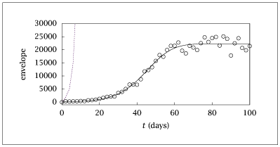
Figure 9.25:

Envelope versus time for hepatitis B virus model; initial guess and estimated parameters fit to data.

Code for Figure 9.25

Text of the GNU GPL.

main.py

  1
  2
  3
  4
  5
  6
  7
  8
  9
 10
 11
 12
 13
 14
 15
 16
 17
 18
 19
 20
 21
 22
 23
 24
 25
 26
 27
 28
 29
 30
 31
 32
 33
 34
 35
 36
 37
 38
 39
 40
 41
 42
 43
 44
 45
 46
 47
 48
 49
 50
 51
 52
 53
 54
 55
 56
 57
 58
 59
 60
 61
 62
 63
 64
 65
 66
 67
 68
 69
 70
 71
 72
 73
 74
 75
 76
 77
 78
 79
 80
 81
 82
 83
 84
 85
 86
 87
 88
 89
 90
 91
 92
 93
 94
 95
 96
 97
 98
 99
100
101
102
103
104
105
106
107
108
109
110
111
112
113
114
115
116
117
118
119
120
121
122
123
124
125
126
127
128
129
130
131
132
133
134
135
136
137
138
139
140
141
142
143
144
145
146
147
148
149
150
151
152
153
154
155
156
157
158
159
160
161
162
163
164
165
166
167
168
169
170
171
172
173
174
175
176
177
178
179
180
181
182
183
184
185
186
187
188
189
190
191
192
193
194
195
196
197
198
199
200
201
202
203
204
205
206
207
208
209
210
211
# [makes] hbv_det.dat

from paresto import Paresto
from misc import octave_save
import numpy as np
import matplotlib.pyplot as plt
import os
from pathlib import Path
plt.ion()

# Define the model
pe = Paresto()
pe.print_level = 1
pe.nlp_solver_options = {'ipopt': {'mumps_scaling': 0}}

pe.x = ['ca', 'cb', 'cc']
pe.p = ['k1', 'k2', 'k3', 'k4', 'k5', 'k6']
pe.d = ['ma', 'mb', 'mc']

def hbv_rxs(t, y, p):
    kr = [10**p.k1,
          10**p.k2,
          10**p.k3,
          10**p.k4,
          10**p.k5,
          10**p.k6]
    rhs = [
        kr[1]*y.cb - kr[3]*y.ca,
        kr[0]*y.ca - kr[1]*y.cb - kr[5]*y.cb*y.cc,
        kr[2]*y.ca - kr[4]*y.cc - kr[5]*y.cb*y.cc
    ]
    return rhs

pe.ode = hbv_rxs

# Measurement weights
mweight = np.sqrt([1, 1e-2, 1e-4])
w = {'a': mweight[0], 'b': mweight[1], 'c': mweight[2]}

def lsq_weighted(t, y, p, w):
    retval = [
        w['a'] * (y.ca - y.ma),
        w['b'] * (y.cb - y.mb),
        w['c'] * (y.cc - y.mc)
    ]
    return retval

pe.lsq = lambda t, y, p: lsq_weighted(t, y, p, w)

# Reaction rate constants
krac = np.array([2, 0.025, 1000, 0.25, 1.9985, 7.5e-6])
thetaac = np.log10(krac)

p_names = pe.p
p_true = {fn: thetaac[i] for i, fn in enumerate(p_names)}

# Output times
tfinal = 100
ndata = 51
tdata = np.linspace(0, tfinal, ndata)
pe.tout = tdata

# Create a paresto instance
pe.initialize()

# Initial condition
small = 0
x0_ac = [1, small, small]

# Simulate using the paresto instance
pin_ac = dict(p_true)
pin_ac['ca'] = x0_ac[0]; pin_ac['cb'] = x0_ac[1]; pin_ac['cc'] = x0_ac[2]
y_ac, zsim = pe.simulate(pin_ac)
y_ac = y_ac.reshape(3, -1)
# Add noise — load from octave-generated file if available (for comparison)
_meas_file = Path('hbv_det_meas.dat')
if _meas_file.exists():
    y_noisy = np.loadtxt(_meas_file, comments='#')  # shape (3, ndata)
    y_noisy = np.maximum(y_noisy, 0)
else:
    np.random.seed(1)
    R = np.diag([0.1, 0.1, 0.1])**2
    noise = np.sqrt(R) @ np.random.normal(0,1,y_ac.shape)
    y_noisy = y_ac * (1 + noise)
    y_noisy = np.maximum(y_noisy, 0)

# Initial guess for rate constants
logkrinit = np.array([0.80, -1.13, 3.15, -0.77, -0.16, -5.46])
p_init = logkrinit.copy()

# Simulate outputs for the initial guess
pin_init = {fn: p_init[i] for i, fn in enumerate(p_names)}
pin_init['ca'] = x0_ac[0]; pin_init['cb'] = x0_ac[1]; pin_init['cc'] = x0_ac[2]
y_init, zsim = pe.simulate(pin_init)

# Initialize parameters
del_value = 1

pe.ic.k1 = logkrinit[0]
pe.ic.k2 = logkrinit[1]
pe.ic.k3 = logkrinit[2]
pe.ic.k4 = logkrinit[3]
pe.ic.k5 = logkrinit[4]
pe.ic.k6 = logkrinit[5]
pe.ic.ca = x0_ac[0]
pe.ic.cb = x0_ac[1]
pe.ic.cc = x0_ac[2]

pe.lb_ub()

for fn in p_names:
    setattr(pe.lb, fn, getattr(pe.ic, fn) - del_value)
    setattr(pe.ub, fn, getattr(pe.ic, fn) + del_value)
# State initial conditions are fixed (lb == ub == ic)

# Estimate parameters
est, y, p = pe.optimize(y_noisy.reshape(3,-1,1))

# Calculate confidence intervals with 95% confidence
conf = pe.confidence(est, 0.95)

print('Initial guess')
print({fn: logkrinit[i] for i, fn in enumerate(p_names)})

print('Estimated parameters')
print('\n'.join(f'{k}: {float(v)}' for k, v in est.theta.items()))

print('Bounding box intervals')
print('\n'.join(f'{k}: {float(v)}' for k, v in conf.bbox.items()))

print('True parameters')
print(thetaac)

# Eigenvalues/eigenvectors of the symmetric Hessian; eigh returns them
# sorted ascending, so column 0 is the weak (poorly-determined) direction.
lam, u = np.linalg.eigh(conf.H)

# Perturb parameters in the weak direction
logkrp = np.array(list(est.theta.values())) + 0.5 * u[:, 0]

# Simulate with perturbed parameters
pp = logkrp
pin_pp = {fn: pp[i] for i, fn in enumerate(p_names)}
pin_pp['ca'] = x0_ac[0]; pin_pp['cb'] = x0_ac[1]; pin_pp['cc'] = x0_ac[2]
yp, zsim = pe.simulate(pin_pp)

# Prepare data for saving
store1 = np.column_stack([pe.tout, y_ac.T, y_init.reshape(3,-1).T, yp.reshape(3,-1).T])
store2 = np.column_stack([pe.tout, y_noisy.T])
# Save store2 first then store1 (matches Octave: save hbv_det.dat store2 store1)
octave_save('hbv_det.dat',
    ('store2', store2),
    ('store1', store1),
)

# Plotting
if not os.getenv('OMIT_PLOTS') == 'true':
    fig, axs = plt.subplots(3, 2, figsize=(12, 10))

    # Plot 1
    axs[0, 0].plot(pe.tout, y_noisy[0, :], '+', label='Noisy Data')
    axs[0, 0].plot(pe.tout, y_ac[0], label='Original Data')
    axs[0, 0].plot(pe.tout, yp[0], label='Simulated Data')
    axs[0, 0].set_xlim(0, 100)
    axs[0, 0].set_ylim(0, 60)
    axs[0, 0].set_title('hbv_det_cccdna')


    # Plot 2
    axs[1, 0].plot(pe.tout, y_noisy[1, :], '+', label='Noisy Data')
    axs[1, 0].plot(pe.tout, y_ac[1], label='Original Data')
    axs[1, 0].plot(pe.tout, yp[1], label='Simulated Data')
    axs[1, 0].set_xlim(0, 100)
    axs[1, 0].set_ylim(0, 600)
    axs[1, 0].set_title('hbv_det_rcdna')

    # Plot 3
    axs[2, 0].plot(pe.tout, y_noisy[2, :], '+', label='Noisy Data')
    axs[2, 0].plot(pe.tout, y_ac[2], label='Original Data')
    axs[2, 0].plot(pe.tout, yp[2], label='Simulated Data')
    axs[2, 0].set_xlim(0, 100)
    axs[2, 0].set_ylim(0, 30000)
    axs[2, 0].set_title('hbv_det_env')

    # Plot 4
    axs[0, 1].plot(pe.tout, y_noisy[0, :], '+', label='Noisy Data')
    axs[0, 1].plot(pe.tout, y_ac[0], label='Original Data')
    axs[0, 1].plot(pe.tout, yp[0], label='Simulated Data')
    axs[0, 1].set_xlim(0, 100)
    axs[0, 1].set_ylim(0, 60)
    axs[0, 1].set_title('hbv_det_cccdnap')

    # Plot 5
    axs[1, 1].plot(pe.tout, y_noisy[1, :], '+', label='Noisy Data')
    axs[1, 1].plot(pe.tout, y_ac[1], label='Original Data')
    axs[1, 1].plot(pe.tout, yp[1], label='Simulated Data')
    axs[1, 1].set_xlim(0, 100)
    axs[1, 1].set_ylim(0, 600)
    axs[1, 1].set_title('hbv_det_rcndap')

    # Plot 6
    axs[2, 1].plot(pe.tout, y_noisy[2, :], '+', label='Noisy Data')
    axs[2, 1].plot(pe.tout, y_ac[2], label='Original Data')
    axs[2, 1].plot(pe.tout, yp[2], label='Simulated Data')
    axs[2, 1].set_xlim(0, 100)
    axs[2, 1].set_ylim(0, 30000)
    axs[2, 1].set_title('hbv_det_envp')

    plt.tight_layout()
    if not os.getenv('OMIT_PLOTS') == 'true':
        plt.show()