Oscillations and Excitability

We now integrate equations (1-3) in Matlab using the following code. First camp.m:

global nu sigma k kt L q h

nu = 0.1;
%nu = 0.04;
sigma = 1.2;
k = 0.4;
kt = 0.4;
L = 10^6;
q = 100;
h = 10;

[T,Y] = ode23('func_camp',[0,2500],[92.366,10,2]);  

figure(1);
hold on;
plot(T,Y(:,1),'b');
plot(T,Y(:,2),'r');
plot(T,Y(:,3),'g');
xlabel('t');
ylabel('\alpha,\beta,\gamma');

Text version of this program Next func_camp.m:

function dy = func_camp(t,y)

global nu sigma k kt L q h

a = y(1);
b = y(2);
g = y(3);

dalpha = nu - sigma*phi(a,g);
dbeta = q*sigma*phi(a,g) - kt*b;
dgamma = kt*b/h - k*g;

dy = [dalpha;dbeta;dgamma];

Text version of this program Finally, phi.m:

function r = phi(alpha,gamma)

global nu sigma k kt L q h

r = (alpha*(1+alpha)*(1+gamma)^2)/(L + ((1+alpha)^2)*((1+gamma)^2));

Text version of this program

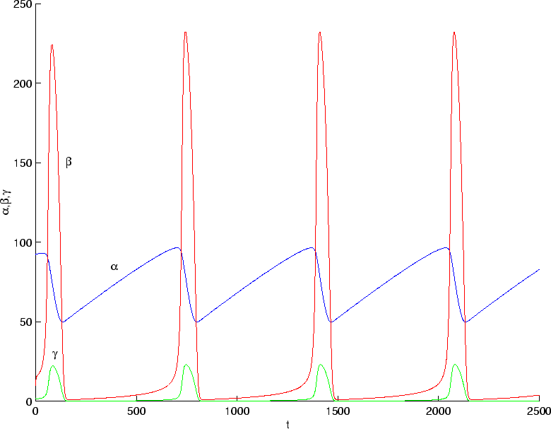
The output from running camp.m is shown in Figure 2 for $\nu = 0.1 s^{-1}$. Here there are sustained, stable oscillations in the three variables.

Figure 2: Oscillations of ATP ($\alpha$), and intracellular ($\beta$) and extracellular ($\gamma$) cAMP for $\nu = 0.1 s^{-1}$.

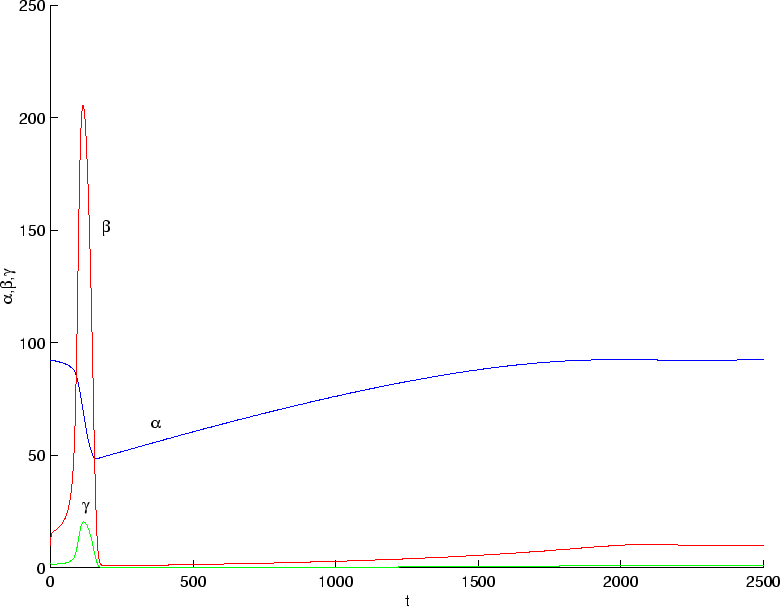
If instead we take $\nu = 0.04 s^{-1}$, corresponding to a lower rate of synthesis of ATP, we find that sustained oscillations are not possible. However, it is still possible to get a single spike of cAMP concentration, as shown in Figure 3. Note that this plot is for the initial conditions $(\alpha,\beta,\gamma) = (92.366,10,2)$. Try varying these initial conditions to see how ``easy'' it is to get such a single spike of cAMP for this model.

Figure 3: A single spike of intracellular ($\beta$) and extracellular ($\gamma$) cAMP for $\nu = 0.04 s^{-1}$.